How to unhide rows in Excel?
This chapter is based on unhiding the rows in Excel. Excel allows the users to hide and unhide the rows of an Excel spreadsheet. When a row is hidden, its data does not display to the users. So, whenever you do not want to show the data of a particular row or column, you need to unhide them.
Excel enables several ways to unhide the rows. For example, you can unhide individual rows, multiple rows, or all hidden rows at once. We will describe all the possible methods in this chapter.
How to know row is hidden?
To unhide any specific row, you should know that which row is hidden. You can go for the row number and check which number is skipped.
For example, if the number 5 6 is not showing between 4 and inside row numbers, it means row5 is hidden. You will also see a double line where a row is hidden.

This can be a hectic and lengthy process to find each hidden row in the entire worksheet. Because, it might be possible that more than one row is hidden at different places. Thus, it will be a time-consuming process to find all the hidden rows one by one.
In that case, you can directly use “unhide all rows” method instead of finding hidden rows. Excel enables the method to enable all hidden rows at once without knowing hidden rows. Hence, you do not need to find and unhide each hidden row one by one.
Methods to unhide rows
Excel offers several methods to unhide the hidden rows in different ways. You can unhide the row however you want, either individual row, all row at once, or only first row. We will discuss the following ones –
- Unhide individual row
- Unhide all hidden rows
- Unhide first row
- Unhide a range of rows
- Unhide the row by increasing row height
Each of these methods works differently to achieve the same result.
Unhide individual row
Sometimes an Excel sheet contains only one or two hidden rows. Hence, it is a good way to unhide the individual row specifically. For this, firstly find that hidden row and then unhide it.
Step to find and unhide hidden row
Step 1: Inside the row header (at the left side of the panel), look for the skipped row number between the two rows.

Tip: You will also see a double line between two rows inside the row header whenever a row is hidden.
Step 2: Keep the cursor on that hidden section in the row header and drag it below.

Step 3: Besides this, you can also right-click to the space between the row header and then choose the Unhide option from the list.

Step 4: You will see that the row that was hidden earlier is now unhidden, and its data is visible as well. Both methods will provide the same result.

Save the new modified Excel sheet to keep the changes permanent. However, this requires each row to be unhidden individually.
Note: In an Excel worksheet, a range of consecutive rows can also be hidden, e.g., rows 5 to 11.
Unhide all rows
Using this method, we can unhide all the hidden rows of an Excel spreadsheet in one go. It saves time and effort to find the hidden rows in entire worksheet and then unhide them one by one.
Follow the steps for this below –
Step 1: Open the targeted Excel sheet, and click on the Select All button (a triangle present between row and column headers).

The entire worksheet will be selected. However, you can click on any cell and then press Ctrl+A to select the entire worksheet.
Step 2: Inside the Home tab, click on the Format dropdown button (present inside the Cells section).

Step 3: Take the mouse over the Hide & Unhide option in this dropdown list and then click the Unhide Rows from another sub dropdown menu.

Step 4: Once you clicked the Unhide Rows here, all the hidden rows will get unhide.

Now, save the modified file by pressing the Ctrl+S shortcut key. Using the same steps, you can also unhide the columns by choosing Unhide columns instead of Unhide rows in the end.
Note: If somewhere rows are hidden in consecutive manner (row 5 to 13), this method does not unhide them. For that type of hidden row, you have to use another method.
Unhide first row
Sometimes, you see that only the first row of an Excel worksheet is hidden. It is a little tricky to unhide the first row or first column because there is no way to select that row or column. However, you can unhide the first row using Unhide all rows’ method, but it unhides all the hidden rows along with the first one. So, if you want only the first row to unhide, this method is not a good choice.
Both above methods will not work here. Thus, we have to look for another method. It is a bit complicated but not so complex too. We will make it easy for you.
We have two methods for it: Namebox and Go To. Both methods are easy and simple.
Using Namebox
We can unhide the first row or column from the Namebox. In case the first row or column is hidden.
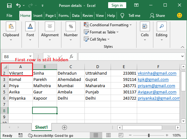
- In our worksheet, see that the first row is hidden.

- In your targeted Excel sheet, go to the Namebox and type A1 to it.

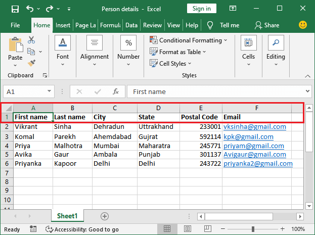
- Now, just press the Enter key, your first hidden row/column will unhide automatically.
Using Go To
Follow the steps to unhide the first row of the Excel sheet using the Go To method.
- Press the Ctrl+G to open the Go To panel like this.

You can also find this option from here Home > Find & Select > Go To. - In the Reference box, type A1 and click OK.

- You will see that your hidden row/column is visible now. This method works for both first row and first column.

Unhide a range of rows
The methods we have discussed till now do not help to unhide rows, which are hidden continuously. For example, four rows between row6 to row 10 are hidden continuously.
For this, Excel enables a different method. Using which you can unhide these types of hidden rows.
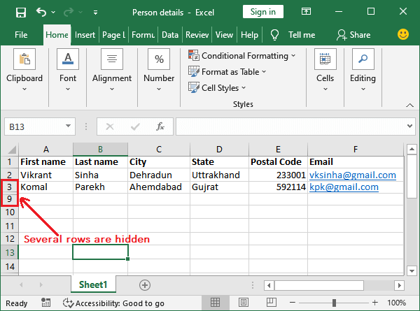
- See in the below screenshot that several rows are hidden here. (Row4 to Row8)
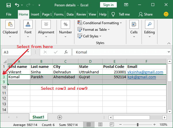
- Hold the Shift key and select two rows: one above the hidden row and another below the hidden row from row header. For example, Row3 and Row9.
- Right-click one of the selected rows and click the Unhide option here.

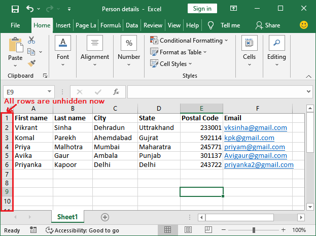
- See that all the rows have been unhide now and the data is also visible.
Tip: If you try to unhide the contiguous hidden rows by selecting and dragging, but it will unhide only a single row at a time.
Unhide hidden rows using row height property
This is one of the best methods to unhide the hidden rows. This method works on all types of hidden rows, such as a single hidden row, several contiguous hidden rows, multiple hidden rows at different places. We will unhide the row by increasing the height of the rows.
Note: This method will all types of hidden rows except the first row.
The default height of the row is 15.0 (20 pixels). So, set the height of all rows to 15.0. See the steps for it below.
Step 1: Click on the Select All button in the Excel worksheet, a triangle between row and column header.

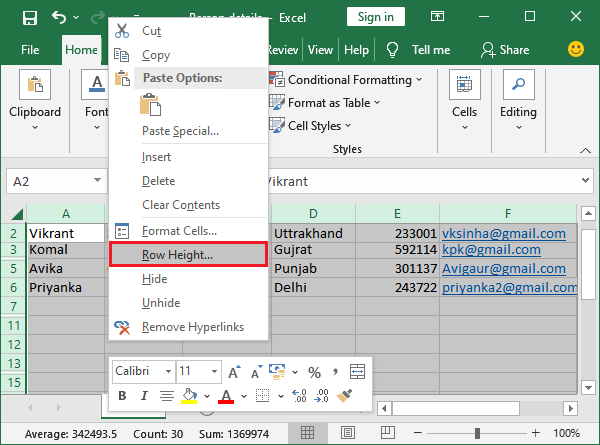
Step 2: Entire sheet has been selected. Now, right-click on it and choose the Row Height option here.
Step 3: A small wizard will open like this where enter the row height 15.0 and click OK.

Now, all the hidden rows are unhidden now except the first row. First row did not unhide.