How to use COUNTIF function in Excel
COUNTIF is one of the commonly used in-built statistical functions in the Excel document. It is used to count the number of cells in a given range that meets criteria (match criteria) in the other cells. For example, count the number of cells that contain numbers, text values, as well as dates.
COUNTIF function includes logical operators (>,<,<>,=) and wildcards (*,?) to match the criteria.
Note: COUNTIF function is not case sensitive means “COA” and “coa” are the same.
In Microsoft Excel, the below syntax is used to use the COUNTIF function –
OR
Where range denotes a range of cells to count, for example, A1:A12
Criteria are used to define the condition that tells the function which cell should be counted, like A2:A5, “John”.
There are the following criteria in which you can apply the COUNTIF function –
Note: COUNTIF function applied for Excel 2000, Excel 2003, Excel 2007, Excel 2010, Excel 2013, Excel 2016, Excel 2019, Excel for Office 365, Excel XP, and Excel 2011 for Mac.
- COUNTIF function for numeric criteria
- COUNTIF function for text
- COUNTIF function with wildcard characters
- COUNTIF function for blank and non-blank cells
- COUNTIF function for greater than, less than, or equal to
- COUNTIF function with the dates
- COUNTIF function for multiple criteria
1. COUNTIF function for Numeric Criteria
COUNTIF function for numeric is used to count cells that are equal to given cells that are greater than or smaller to a given range.
Syntax for Numeric Criteria
The below formula is used to apply the COUNTIF function for numbers –
Steps to use COUNTIF function for Numeric Criteria
There are the following steps to use the COUNTIF function in Excel –
Step 1: Go to the bottom of the Search bar, type Microsoft Excel on it, and then press Enter key from the keyboard. A Microsoft Excel document will appear on the screen.
Step 2: Click on the File -> New -> Blank document -> Create to open a new blank document. Click on the File -> Open -> Browse desired file location -> Open button to open your desired existing Microsoft Excel document.

Note: In this example, we use a New Microsoft Excel document.
Step 3: Prepare a list of data in which you want to apply the COUNTIF function. (In our case, data starts from cell B2 and ends in cell B7. See the below screenshot.)

Step 4: Place mouse pointer on the cell where you want to apply the COUNTIF function. Type formula =COUNTIF(B2:B7,”40″) in the selected cell. (we want to count the number of cells that contains number 40)

Step 5: Press the Enter key from the keyboard. The screenshot below shows the result in the selected cell. (In our case, COUNTIF function returns value 2 because the value 40 present twice (cell B2 and B5) in the given data)

Method 2: COUNTIF function for text criteria
Microsoft Excel also allows us to count the number of cells that contain similar text.
Syntax
To use the COUNTIF function in the Microsoft Excel, follow the below given syntax:
Steps to use COUNTIF function for text criteria
There are the following easiest steps to use the COUNTIF function for text criteria –
Step 1: Double click on the Microsoft Excel icon to open the Microsoft Excel document.
Step 2: Click on the File -> New -> Blank document -> Create to open a New Excel document. Click on the File -> Open -> Browse file location -> Open to open the existing Microsoft Excel document.

Note: In our case, we are going to open an existing Microsoft Excel document.
Step 3: Prepare a list of data on which you want to apply the COUNTIF function. See the screenshot given below.

Step 4: Place the cursor in the selected cell and type formula =COUNTIF(B1:B9,”Alice”) in the cell, where you want to see the result of the COUNTIF function.

Note: In this example, we want to see the occurrence of string Alice in the given data.
Step 5: Once the COUNTIF function is completed, press the Enter key from the keyboard.
The below-given screenshot shows the result of the COUNTIF function in your selected cell.

Method 3: COUNTIF function with wildcard characters
Wildcard character includes question mark (?), asterisk (*), and tilde (~) symbols to match the criteria. In Microsoft Excel, asterisk matches zero and more characters.
The below syntax is used to apply the COUNTIF function in the Excel document –
Steps to use the COUNTIF function with wildcard characters
Step 1: Open a new or an existing Microsoft Excel document in which you want to apply the COUNTIF function.
Step 2: Place mouse pointer in the cell and type formula =COUNTIF(B1:B9,”*Alice*”) in the selected cell.

Step 3: Press the Enter key from the keyboard. You can see that the COUNTIF function returns the cells that contain similar text.
Method 4. COUNTIF function for blank and non-blank cells
COUNTIF for non-blank cells function is fully automatic, easy to use, time-saving, and also produces the instant result for a given data set. It is used to count numbers or text ranges of any columns without considering the blank cells.
Syntax:
The below syntax is used to count the number of blank cells in Microsoft Excel –
The below syntax is used to count non-blank cells in Microsoft Excel –
Steps to use the COUNTIF function
A list of steps to use the COUNTIF function for blank and non-blank cells is as follows –
Step 1: Create a new blank Microsoft Excel document or open a new existing document.
Step 2: Place mouse pointer on the cell in which you want to show the result.
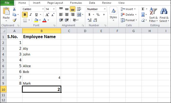
Step 3: Type or copy-paste the given formula =COUNTBLANK(B2:B9) in your selected cell to see the result of the COUNTIF function. In our case, cell B10 contains the formula.

Step 4: Once the COUNTIF formula is completed strike the Enter key from the keyboard. You can see that the result (number of blank rows) will appear in your selected cell.

Method 5. COUNTIF function for greater than, less than, or equal to
1. Syntax for greater than
2. Syntax for greater than equal to
3. Syntax for less than
4. Syntax for less than equal to
5. Syntax for equal to
Steps to apply COUNTIF Function
Step 1: Create a new blank Microsoft Excel document or open an existing document.
Step 2: Place mouse pointer on the cell in which you want to show the result.
Step 3: Type or copy-paste the given formula =COUNTIF(A1:A9,”>5″) in your selected cell to see the result of the COUNTIF function. (In our case, cell B10 contains the given formula).

Note: In this example, we are going to check greater than condition. You can also check other conditions like greater than equal, less than, less than equal to, and equal to based on your requirement.
Step 4: Once the COUNTIF formula is completed, strike the Enter key from the keyboard. You can see that the result (number of cells greater than 5) will appear in your desired cell.

Method 6: COUNTIF function with the dates
Microsoft Excel allows us to count the number of cells that contain date greater than, less than or equal to a specified date as well as current date.
Follow the below-given syntax to use the COUNTIF function with dates –
1. Count the cells that contain dates equal to a specified date.
2. Count the cells that contain dates greater than or equal to a specified date.
3. Count the cells that contain dates less than or equal to a specified date.
4. Count the number of cells that contain a date equal to the current date.
5. Count the number of cells that contain a date greater than the current date.
6. Count the number of cells that contain a date greater than the current date.
Steps to use the COUNTIF function with the dates
Step 1: Go to the bottom of the Search bar, type Microsoft Excel on it, and then press Enter key from the keyboard. A Microsoft Excel document will appear on the screen.
Step 2: Click on the File -> New -> Blank document -> Create to open a new blank document. Click on the File -> Open -> Browse desired file location to open your desired Microsoft Excel document.
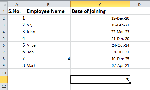
Step 3: Select the cell in which you want to apply the COUNTIF function for dates and type given formula =COUNTIF(C2:C10,”<“&TODAY()) in the selected cell as shown in the screenshot given below.

Note: In our case, we are going to count the number of cells that contain dates greater than today.
Step 4: Press the Enter key from the keyboard. The screenshot below shows the result in the selected cell.

Method 7: COUNTIF function for multiple criteria
Microsoft Excel also allows us to use the COUNTIF function for more than one criteria.
The below syntax is used to apply the COUNTIF function in an Excel document.
Steps to use the COUNTIF function
Step 1: Go to the bottom of the Search bar, type Microsoft Excel on it, and then press Enter key from the keyboard. A Microsoft Excel document will appear on the screen.
Step 2: Click on the File -> New -> Blank document -> Create to open a new blank document. Click on the File -> Open -> Browse desired file location to open your desired Microsoft Excel document.
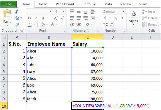
Step 3: Select the cell in which you want to apply the COUNTIF function for dates and type given formula =COUNTIFS(B2:B9,”Alice”,C2:C9,”>15,000″) in the selected cell as shown in the screenshot given below.

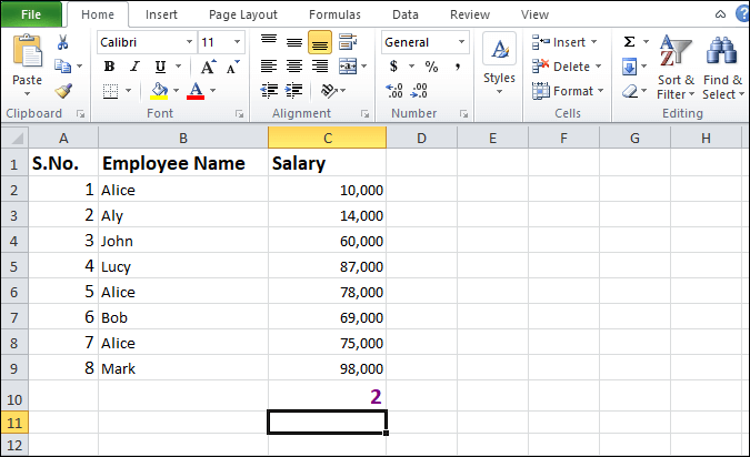
Step 4: Once the formula is completed, press the Enter key from the keyboard. The screenshot below shows the result of the COUNTIF function for multiple criteria.


