
How to Calculate IRR in Excel?
In Excel, the IRR function is a financial function that returns the internal rate of return (IRR) for a series of cash flows at regular intervals.
What is IRR?
The internal rate of return (IRR) is the discount rate that makes the net present value equal to zero. When the IRR has only one value, this criterion becomes more interesting when comparing different investments’ profitability. In Excel, IRR has the following calculation formula:
The IRR function uses the following arguments:
1. Values (required argument): This is an array of values representing the series of cash flows. Cash flows include investment and net income values. Values can be a reference to a range of cells containing values.
- The value argument should contain at least one positive and one negative value to calculate the return’s internal rate.
- Those values are ignored if the array or reference argument contains logical values, empty cells, or text.
- IRR in Excel interprets the order of cash flows based on values; the values should be in sequential order.
- The cash flows do not necessarily have to be even, but they must occur at regular intervals, for example, monthly, quarterly, or annually.
2. Guess (optional argument): This is a number guessed by the user that is close to the expected internal rate of return (as there can be two solutionsfor the internal rate of return).
- Excel uses an iterative technique for calculating IRR. Starting with the guess, IRR cycles through the calculation until the result is accurate within 0.00001 percent. Suppose IRR can’t find a result that works after 20 tries, the #NUM! The error value is returned.
- In most cases, you do not need to provide a guess for the IRR calculation. If the guess is omitted, it is assumed to be 0.1 or 10 %.
- Suppose IRR gives the #NUM! Error value, or if the result is not close to what you expected, try again with a different value for guess.
IRR Function in Excel
The problem with using math to calculate the internal rate of return is that the necessary calculations are complicated and time-consuming.
A math-based solution involves calculating the net present value (NPV) for each cash flow amount using various guessed interest rates on a trial-and-error basis. Then, those NPVs are added together. This process is repeated using multiple interest rates until you find the exact interest rate that produces NPV amounts that sum to zero. The interest rate that produces a zero-sum NPV has then declared the internal rate of return.
To simplify this process, Excel offers three functions for calculating the internal rate of return. Each of these represents a better option than using the math-based formulas approach. These Excel functions are:
- IRR Function: IRR function calculates the internal rate of return for a series of cash flows, assuming equal-size payment periods.
- XIRR Function: The XIRR function calculates a more accurate internal rate of return because it considers different-size time periods.
To use this function, you must supply both the cash flow amounts and the specific dates on which those cash flows are paid. - MIRR Function: The MIRR function (modified internal rate of return) works similarly to the IRR function, except that it also considers the cost of borrowing the initial investment funds and compound interest earned by reinvesting each cash flow.
The MIRR function is flexible enough to accommodate different interest rates for borrowing and investing cash. Because the MIRR function calculates compound interest on project earnings or cash shortfalls, the resulting internal rate of return is usually significantly different from the internal rate of return produced by the IRR or XIRR function.
How to Calculate IRR
To understand how to use the IRR function in excel, follows the following steps:
Assuming you have been running a business for three months and now you want to figure out the rate of return for your cash flow.
Step 1: Type the initial investment into B2 cell. Since it is an outgoing payment, it needs to be a negative number.
Type the subsequent cash flows into the cells under or to the right of the initial investment. This money has been coming in through profit, so we enter these as positive numbers.
Here is the created report in which we expect to profit at the end of the months.
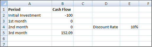
The discount rate equals 10%. This is the rate of return of the best alternative investment.
Step 2: In Excel uses the NPV function to calculate the present value of a series of cash flows and subtracts the initial investment.

A positive net present value indicates that the project’s rate of return exceeds the discount rate. In other words, it’s better to invest your money in the project than to put your money in a savings account at an interest rate of 10%.
Step 3: The IRR function below calculates the internal rate of return of the project.
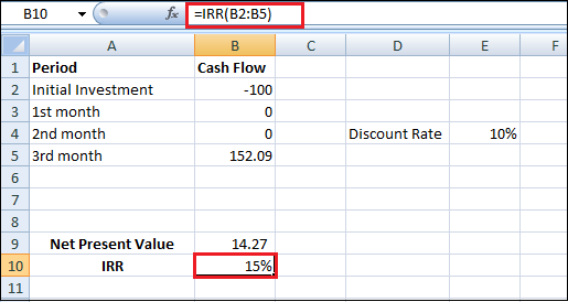
Step 4: The internal rate of return is the discount rate that makes the net present value equal to zero. You need to replace the discount rate of 10% in cell E4 with 15%.

A net present value of 0 indicates that the project generates a return rate equal to the discount rate. In other words, investing your money in a project or putting your money in a high-yield saving account at an interest rate of 15% yields an equal return.
Present Values
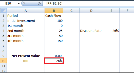
Let’s suppose another project requires an initial investment of Rs.100. We expect a profit of Rs.25 at the end of the second month, Rs.50 at the end of the third month, and Rs.152.09 at the end of the fourth month as given below:
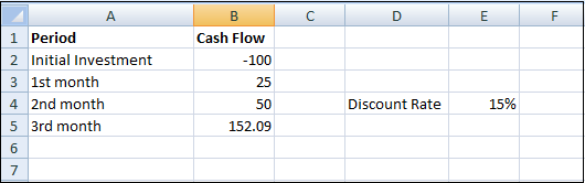
Step 1: Now, use the NPV function to calculate the present value of a series of cash flows of this project.

Step 2: The IRR function calculates the internal rate of return of this project.

Step 3: Again, the internal rate of return is the discount rate that makes the net present value equal to zero. You need to replace the discount rate of 15% in cell E4 with 39%.

A net present value of 0 indicates that the project generates a return rate equal to the discount rate. In other words, you are investing your money in this project or putting your money in a high-yield saving account at an interest rate of 39% yield an equal return.
Step 4: First, we calculate the present value (Pv) of each cash flow. Next, we sum these values as given below.

Instead of investing $100 in this project, you could also put Rs.17.95 in a savings account for 1st month, Rs.25.77 in a saving account for 2nd month, and Rs.56.28 in a saving account for 3rd month, at an interest rate equal to the IRR (39%).
IRR Rule
The IRR rule says that you can accept the project if the IRR is greater than the required return rate. IRR values are frequently used to compare investments. In the below example, we take A and B two different projects.
Step 1: The IRR function calculates the internal rate of return of project A.
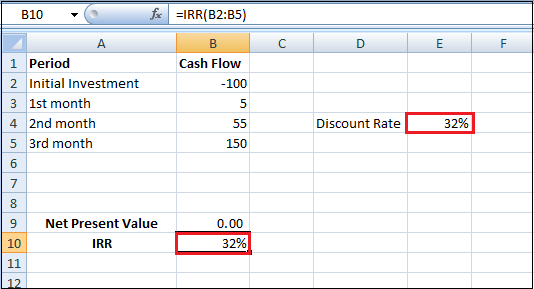
If the required rate of return equals 15%, you should accept this project because the IRR of this project equals 32%.
Step 2: The IRR function calculates the internal rate of return of project B.
In general, a higher IRR indicates a better investment. Therefore, project A is a better investment than project B.


