
Excel match function
MATCH function is an in-built Excel function that allows the users to locate the position of a lookup in a row, column, or table. You can also understand it as – MATCH function searches for a specified item in a range of cells and returns its position to the user.
For example, An Excel column contains four values 34, 12, 53, 29, respectively A1:A4. To find the position of 53 in within a range A1:A4, the MATCH formula will be –
=MATCH(53, A1:A4, 0)
After finding 53 within the specified range, it will return 3, which means that the 53 is the third item in the range.
Note: MATCH() function supports the exact match, approximation match, as well as wild card (*, ?) match.
The MATCH() function is an alternative to the LOOKUP function. Always use the MATCH function when you need to find the position of an item within a range (range: specified by user) instead of that item itself.
Syntax and Parameters
Following is the syntax and parameter values for the MATCH function –
“MATCH() function is not case-sensitive, so Happy and HAPPY both are same for it. “
LOOKUP_value (required)
LOOKUP_value parameter consists of a value to be searched in a specified range of cells in an Excel worksheet. This parameter is a required parameter, which means the value must be passed in this argument. It can accept numbers, text, or logical values.
For example, you are looking for someone’s date of birth by using the name of the person as LOOKUP_value. Hence the date of birth is the value you want.
Note: Text value must be enclosed between double-quotes (“”).
LOOKUP_range (required)
LOOKUP_range is a parameter that contains the range within which the LOOKUP_value will be searched. For example, the range will be specified as A1:A10. This is the range on which you will look for the matching value.
match_type (optional)
Unlike the above two parameters, it is an optional parameter that accepts a numeric value. The number can be either 1, 0, or -1 and the default value is 1 for this parameter.
- 1 for exact or next smallest match
- 0 for an exact match
- -1 for exact or next largest match
This parameter specifies how Excel will search for the position of LOOKUP_value within the LOOKUP_range array parameter.
Return value
- MATCH() function returns the position of the value if found in the specified range of cells.
- In case the MATCH() function does not find the specified value, it returns #N/A error.
Important tips:
Following are some important tips that need to be noticed for the MATCH() function:
- MATCH() function returns the position of the searched element. Remember not the value itself.
- If the MATCH() function is unable to find the value within the specified range, it returns #N/A error code.
- If you are searching for the text data, pass the value in double-quotes as a LOOKUP_value. E.g., “Bluetooth” within the range A2:A15.
- While matching text value, MATCH() function looks for the exact spelling to find a match. It is not case-sensitive, so it is not able to distinguish between UPPERCASE and lowercase letters.
- This function starts counting the position for the specified item from the range you provide in the function rather than from the A1 cell. Hence, if you change the range, return position will also change.
- If the lookup_value is a text string and you are also using the third parameter match_type value as 0. You can also use a wildcard character in it.
- ? (question mark) to match any single character in the text string.
- * (asterisk) to match a pattern or sequence of characters inside a text string.
- ~ (tilde operator) is a special operator that is before the character to find an actual question mark (?) or asterisk (*) character used in the string.
Now, let’s see different examples for this function to understand it better practically.
How MATCH() function is used in Excel?
To understand the working of the MATCH() function, how differently it works with different parameter values, we have several examples as discussed below.
It is helpful when we have too large dataset in Excel and want to find something in that. You can look for the position by using a particular word in the MATCH() function. If the value exists in that Excel worksheet, the MATCH() will return the position of it.
Then, you can directly go for it and see the complete information. It saves the time of users in searching data.
Note: Remember that – this function start counting the position for the specified item from the range you defined in the function, not from the A1 cell. Hence, if you change the range, the position return by it will also change.
Exact Match Example
Firstly, we will discuss two examples for exact matching on string data. See the examples below:
Example 1: Find the String data
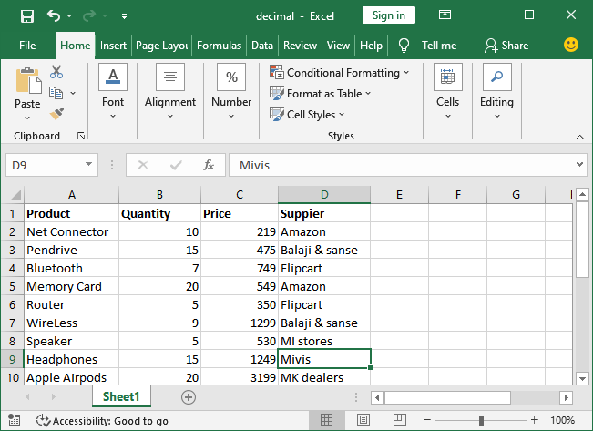
Suppose we have this set of product data given below in which we will look for Boat earphone position.
See the following steps how could it be done:
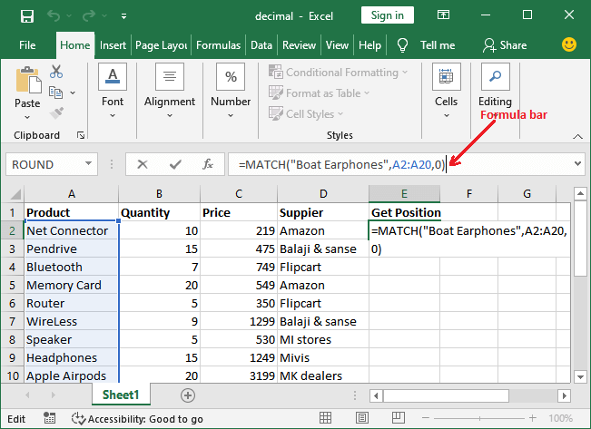
Step 1: Select a cell to store the returned result and write the following formula in the formula bar.
=MATCH(“Boat Earphones”,A2:A20,0)
Here Boat Earphones is the lookup_value to be searched within A2 to A20 range and 0 is used for exact matching.
Step 2: By pressing the Enter key, a position of the searched keyword will return if it exists.
Result when LOOKUP_value found
Step 3: See the position returned by the MATCH() function after finding Boat earphones in the Excel file.

Result when LOOKUP_value is not found
Now, we will look for a value that is not available in the Excel sheet. For example, handset within the A1 to A10 range.
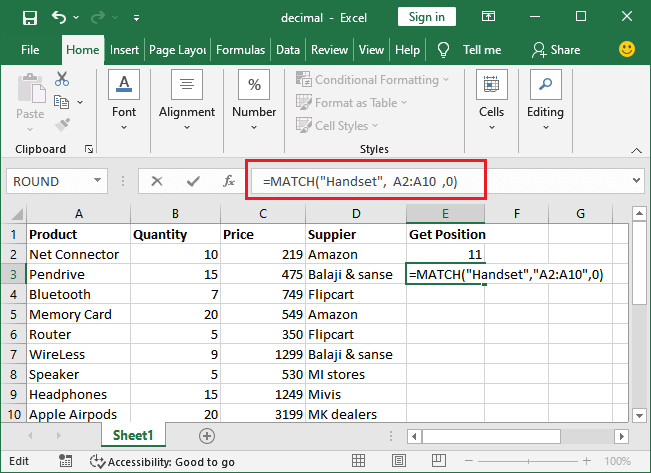
Step 4: In case the LOOKUP_value is not found in the target range of cells, it will not return any position. It will return #N/A error in the cell, as showing in the below screenshot.

Example 2: Lookup for the position of planet
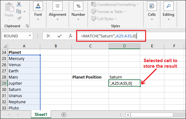
Let’s see a simple example of searching the position of the planet. We have a list of planets in which you can find the position of a particular planet using the MATCH() function.
We need to find an exact match, not an approximate value. So, we will use 0 as the third parameter value for exact matching.

Step 2: Copy and paste the following MATCH() formula in your Excel formula bar.
=MATCH(“Saturn”,A25:A35,0)
Here Saturn is the lookup_value to be searched within A25 to A35 range and 0 is used for exact matching.
Step 3: Now, click the Enter key of your keyboard and see the position returned by the MATCH() function after finding the exact match to Saturn.
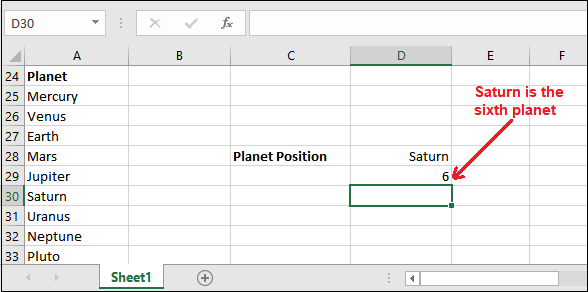
The returned value is 6, which means that Saturn is the sixth planet in the list.
Approximation Match
Now, using the following examples, we will look for the exact or approximate matches. Thus, you will see how the MATCH() function works to find the position through an approximate match.
There are two ways: One is the next smallest match and another is the next largest match. Describe one-one example for both methods.
Example 1: Next Smallest match
Now, we will show an example of an approximation match by using 1 (for the next smallest match) in the third parameter of the MATCH() function. In this example, we will take numeric dataset.
We have this numeric set of data in an Excel worksheet.
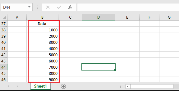
We will lookup for the exact as well as approximate value from the Data column using the MATCH() function. Follow the steps below:
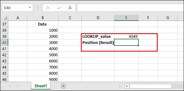
Step 1: We are looking for 4349 or approximate value in the following data available.

Step 2: Use the following formula on your Excel worksheet in the Formula bar and get the result by clicking the Enter key.
=MATCH(4349,B38:B50,1)

Step 3: See that the MATCH() function returned 4 as position in the specified range. Value 4349 is not present in the specified range; it is nearest to the 4000. Hence, it has returned the approximate value position, i.e., 4.

This is the example of finding the position of the exact or next largest approximate value.
Example 2: Next Largest match
Now, we will show an example of an approximation match by providing -1 (for the next Largest match) in the third parameter of the MATCH() function. For this example, we will the same dataset used in previous example.
We have this numeric set of data in an Excel worksheet.

We will lookup for the exact as well as the next largest approximate value from the Data column using the MATCH() function. Follow the steps below:
Step 1: We are looking for the same value, 4349 and find its exact or approximate match in the following data available.
Step 2: Use the following formula on your Excel worksheet in the Formula bar and get the result by clicking the Enter key.
=MATCH(4349,B38:B50,-1)
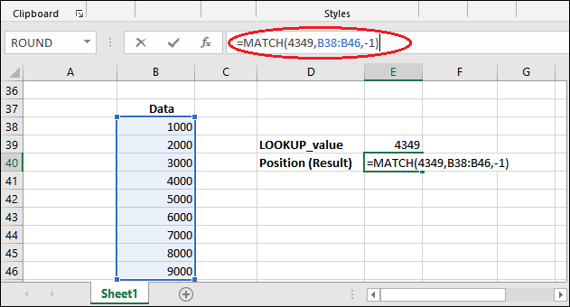
Step 3: See that the MATCH() function returned 5 as position in the specified range. Value 4349 is not present in the specified range; it is the next largest to the 5000. Hence, it has returned the approximate value position, i.e., 5.
This is the example of finding the position of the exact or next largest approximate value.
Example 3: Wildcard match
Excel allows the users to perform wildcard match on data by using the MATCH() function. You can perform two wildcard operations in Excel: one using asterisk (*) and question mark (?) operator. We will show the example of wildcard matching with the help of MATCH() function.
We have this set of data in an Excel worksheet on which we will perform wildcard matching on data.

Using Question mark (?) operator
We will look for a pattern using a question mark (?) symbol with the text string inside the MATCH() function. For example, Spe??er. The MATCH() function will look for text containing a word similar to it, like Speaker.
Step 1: Select a cell to store the result and write the following MATCH() formula. It will look for the match having P?ndrive in the Product column.
=MATCH(“P?ndrive”,A1:A15,0)
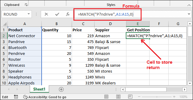
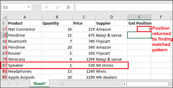
It will return the position of the first match found in the Product column. Remember that question mark (?) will ignore the second letter of the specified text.
Step 2: It has returned position 3 when it gets the first match.

Using Asterisk (*) operator
We will look for a pattern using asterisk (*) symbol with the text string in MATCH() function. For example, Sp*. The MATCH() function looks for text which contains Sp in the beginning.
Step 1: Select a cell to store the result and write the following MATCH() formula. It will look for the match having Sp at the beginning of the Product name.
=MATCH(“Sp*”,A1:A15,0)

It will return the position of the first matching pattern in the Product column. Remember that asterisk (*) operator leads to the pattern specified in the text string.
Step 2: It has returned position 7 on finding the first match.
What if data does not match
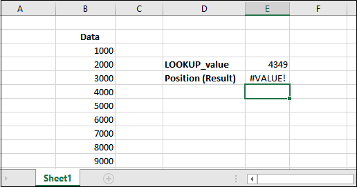
Excel generates an error (#N/A) when the MATCH() function does not find the specified value. This #N/A error refers to Value Not Available Error. See the below screenshot for the following MATCH() operation for value not available.
In the given set of data, we are searching for a value of 4349 within the B38 to B50 range. Let’s see what the MATCH() function for #N/A result.

See that the 4349 value did not find within the specified range. So, it has been returned #N/A error, i.e., Value Not Available Error.


