
Cell Styles in Excel
MS Excel or Microsoft Excel is powerful spreadsheet software with a distinct range of built-in features and functions. It can handle vast amounts of data and supports various formatting options for data recorded within the spreadsheets. Excel has different formatting options to format our worksheets quickly, from simply copying the formatting from other cells to predefined conditional formatting. Apart from this, Cell style is another wonderful feature for formatting Excel cells within the sheets.

This article discusses the brief introduction of Cell Styles in Excel and the step-by-step tutorial to apply predefined Cell Styles and create custom Cell Styles in Excel.
What is Cell Style in Excel?
A cell style refers to a combination of many formats or attributes that we can apply within the Excel cells. Although we can apply each combined formatting separately, it will take more time. Instead of using various formatting separately, we better apply a single style to simultaneously implement a collection of formats. A cell style is a quick way to change the appearance of the sheet efficiently.
A cell style can combine preferences for the six attributes described below:
- Fonts (type, color, and size)
- Alignment (vertical and horizontal)
- Number Format
- Pattern
- Borders
- Protection (locked & hidden)
We can combine the above formats into a single cell style. For example, we can create a style that includes settings for a specific font color, a cell background color, and italic font style, a cell border, and a number format. Whenever we need to use such a combination of formatting, we can quickly apply them all by simply selecting the style we created instead of applying each format one by one. It helps us apply multiple formats at once with a few clicks quickly and adds consistency to the overall look of the worksheet.
How is a cell style helpful in Excel?
Although cell styles in Excel are not as powerful as Word, they are helpful and save time to apply complex formatting within the sheet quickly. For example, consider that we have entered some data to around forty to fifty cells with the font size of 12 pt. But, later, we realized that we needed to use the font size of 16 pt. in all those cells instead of 12 pt. In such a case, we can edit the cell style and put the font of 16 pt., rather than editing the font size of each corresponding cell. All the cells with that specific style will automatically change to the font size of 16 pt.
Likewise, we can also modify the other attributes (such as font type, color, size, number format, borders, vertical and alignment, etc.) through a cell style.
How to use Cell Styles in Excel?
Excel typically offers two efficient options to use cell styles on a selected cell or a range of multiple cells. We can either use any of the existing cell styles installed within Excel or create our custom style manually by choosing specific fonts, colors, shades, etc.
An existing cell style is the combination of formatting options already created and ready for us to use to desired cell or range of cells. Excel has a wide range of existing cell styles divided into different types: Normal, Bad, Good, and Neutral. Furthermore, the styles are divided based on different data types as well. For example, Data and Model. The existing cell styles cover almost everything from titles and headings to color in different elements and accents to currency and number formats.
We need to perform the following steps to use or apply existing/ predefined cell styles in Excel:
- First, we need to select the specific cell or a range of multiple cells to which we wish to apply the style.
- After selecting the desired cells, we need to go to the Home tab and click on the drop-down icon associated with the ‘Cell Styles‘ option under the Styles

- Clicking on the Cell Styles drop-down icon will launch a pop-up window, as shown below:
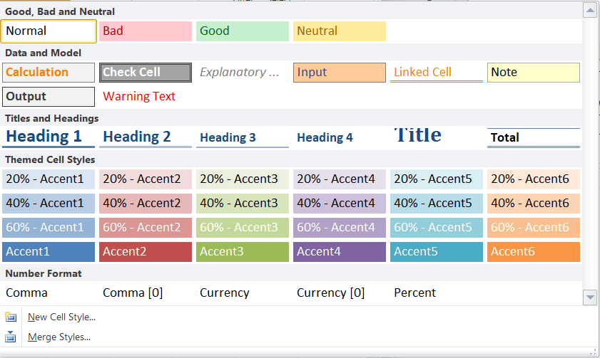
In the above image, these are the existing cell styles in Excel. We can click on the desired cell style, and the same will be instantly applied to the selected cell or range within the active sheet. Apart from this, we can also check the live preview of any particular style by moving the mouse pointer over it. As soon as our pointer hovers on a specific style, Excel displays the corresponding style temporarily on the selected cell or a range.
In this way, we can apply existing or default cell styles in Excel.
How to create a Cell Style in Excel?
Although Excel has several default cell styles, we may sometimes need our specific style to use in any particular workbook. We can create a custom cell style with desired settings for each corresponding format within the style. Whenever we want to use our custom style, we can select it and reuse it like the Excel default cell styles.
We need to perform the following steps to create a custom cell style in Excel:
- First, we need to select a cell or a range of cells.
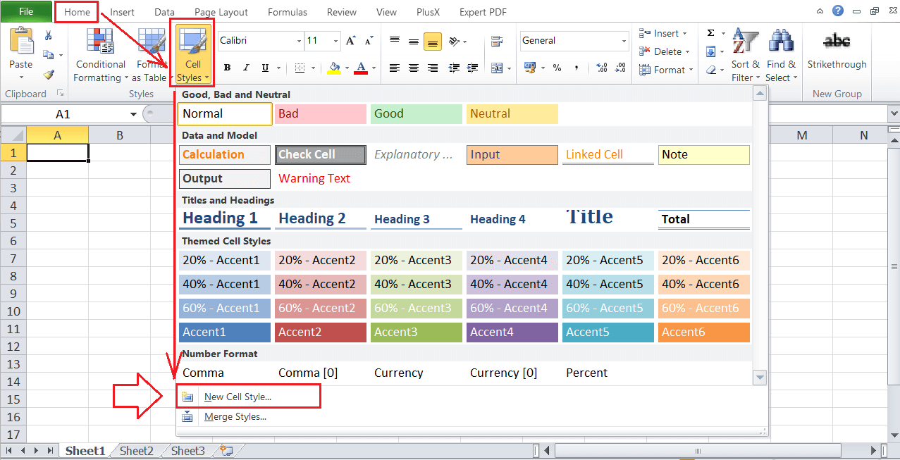
- Next, we need to go to the Home > Cell Styles and click on the ‘New Cell Style‘ option, as shown below:
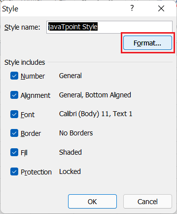
- In the next window, Excel displays the existing preferences of applied style. We can enter a name for our style at the top of the window next to the ‘Style name‘. After entering the name for our custom style, we need to click on the ‘Format‘ button to specify formatting preferences.

- After clicking the Format button from the Style window, we will see the Format Cells dialogue box. In the Format Cells dialogue box, we need to go through all the tabs and choose the desired preferences like the number, font, border, etc.

We selected the green background in the above image with automatic pattern color and dotted pattern style. - After choosing the desired preferences through different tabs, we need to click the OK It will again move us back to the Style window, as shown below:

In the above image, we can notice that the preferences in the style window have changed from the earlier ones. Now, it displays the preferences that we choose from the Format Cells dialogue box. - After verifying the selected formatting preferences from the Style window, we need to click on the OK button to save our custom style in the active workbook. We can uncheck the checkbox of any format settings we don’t want to use from the Styles window before clicking on the OK button.
- After creating the custom style, we can access the same by going to Home > Cell Styles > Custom. We will get our saved styles at the top of the style selection window under the Custom option, as shown below:
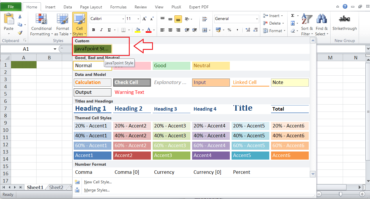
We can click on our created style, and it will be applied to the selected cells within the current workbook.
Note: When we create a custom style in Excel, the style is saved within the workbook. This means that we can access our created style in all the sheets of the current workbook only, not on other workbooks.
How to merge or export cell styles from one Workbook to another?
As discussed above, the custom cell style we create is saved within the respective workbook only. Therefore, we need to merge cell styles to use the same style with other workbooks, which typically copies the applied style from one workbook to another.
We can perform the following steps to merge or export cell style from one workbook to another:
- First, we need to open both the workbooks: the one from which we want to copy/ merge cell style and another to which we want to apply the style.
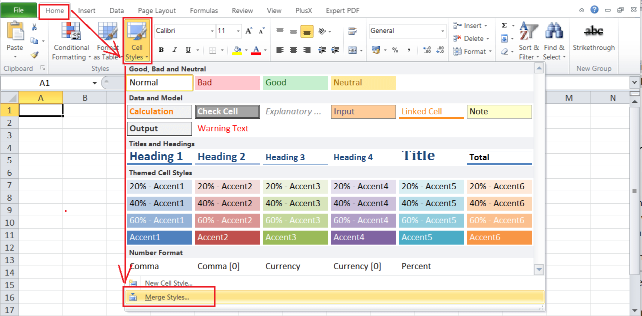
- Next, we need to go to the workbook to which we are going to apply a style. After that, we must navigate the Home > Cell Styles and click on the ‘Merge Styles‘ option, as shown below:
- After clicking on the Merge Style option, Excel displays a list of other workbooks running in the background. We can select the workbook name from which we want to merge the style into our current workbook. After selecting the desired workbook, we must click the OK
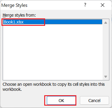
In the above image, we are merging the style from Book1.xlsx to Book2.xlsx.
After merging the style into our desired workbook, we can access it from Home > Cell Styles > Custom.

How to Edit a Cell Style?
Excel also enables users to edit the cell styles as per their choice. We can edit our custom styles as well as the existing styles in Excel. For this, we need to go through the following steps:
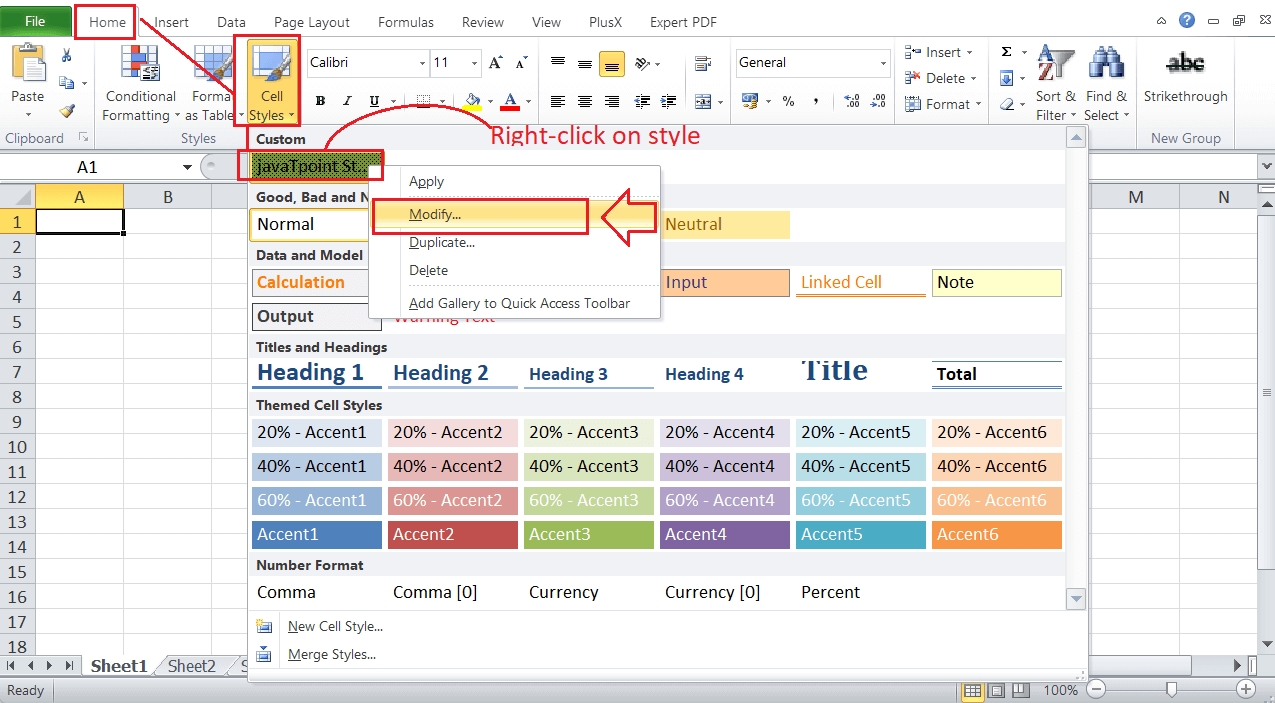
- First, we need to go to Home > Cell Styles and press the right-click button on the style we want to edit. Next, we must click the Modify option from the list, as shown below:
- After clicking the Modify option, Excel launches the Style window and displays the current preferences of formatting saved in the corresponding style. Since we want to edit the style, we need to click the Format button from the Style window.
- In the Format Cells dialogue box, we can change formatting using their respective tabs within the Format Cells window. Once we have edited the formatting preferences, we need to click the OK button to return to the Style window.

- Lastly, we need to click the OK button from the Style window to save all the changes within the selected style. We can also input a new name for the modified style before clicking the OK button.

Similarly, we can use the other options from the right-click menu list to perform related actions, such as applying a style, duplicating it, deleting a style, etc.

How to remove/ clear Cell Styles in Excel?
If we don’t like the style or we want to remove the applied style from our workbook completely, it only takes a few steps to follow.
First, we need to select all those cells or a range of cells from which we are willing to remove the applied style. Next, we need to go to the Home tab and click the Cell style icon. In the next window, we need to click the ‘Normal‘ style located near the top under Good, Bad and Neutral. It looks like this:
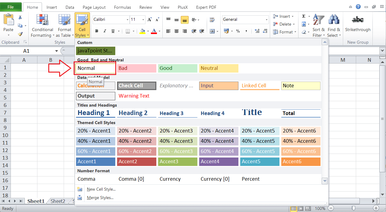
Clicking on the ‘Normal’ option removes any applied style from the selected cells within the active workbook.
Quick Keyboard Shortcuts for Cell Styles
The keyboard key combination or shortcut is the fastest way to access any specific features or commands in Excel. Excel has predefined shortcuts for most of the built-in features. Unfortunately, we don’t have any definite key combination for cell styles in Excel. However, the Alt key method works perfectly.
Whenever we press the Alt key while the Excel window is active, we activate the quick shortcut keys of Excel tools or commands. Excel then displays specific key (s) on built-in tools within the active window. We only need to press the combination of keys one after another to move through Excel tools or features sequentially.
To access the cell styles in Excel, we need to use the Alt key followed by the ‘H’ and ‘J’ keys, i.e., “Alt + H + J”. The Alt key activates the quick shortcuts keys, the H key navigates the Home tab, and the J key selects the Cell Styles option from the ribbon.

After pressing the shortcut key combination, we can use the arrow keys to select the desired style and hit the Enter key to apply.
For other cells styles options, we need to use the following shortcuts:
| Action | Shortcut Key |
|---|---|
| New Cell Style | Alt + H + J + N |
| Merge Style | Alt + H + J + M |


