
How to Split Cells in Excel
MS Excel or Microsoft is the popular spreadsheet program that most people use for different tasks. Sometimes, we may get the wrongly formatted data while downloading it from the web or getting it extracted from other software. The typical case is when we have different data in the same cell that must be broken up into different cells. The data may be separated by a comma, semicolon, tab, or any other character. In such situations, we need to split the cells in Excel. For example, we might have full names of people in a single cell, and we may need to split these into first names and the last names in consecutive columns.
In this article, we are discussing three simple methods that help us to split cells in Excel, such as:
- By using the Text to Columns Feature
- By using the Flash Fill Feature
- By using the Excel Text Functions
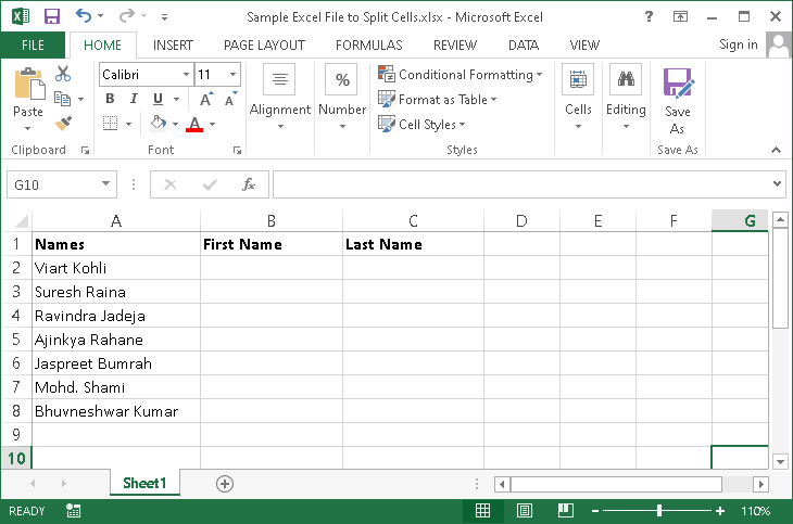
In all of the above methods, we will use the following data set as an example, where we have a single cell with two different items (First Name, Last Name) separated by a comma:
Let us discuss each method in detail:
Split Cells in Excel Using Text to Columns
One of the simplest and commonly used methods to split cells in Excel includes using the Text to Columns tool. This method allows us to split the whole columns with all cells using the desired rules of separating the data. The tool can easily separate the data of the cells, whether the separating text is a comma, space, tab, etc.
Although this particular method is the best way to split cells in Excel, we need to try other ways to split hundreds or thousands of cells. Depending on the data, one method may produce better results than others. The lower the level of data consistency, the more difficult the process becomes.
The method of splitting a cell using the Text to Columns tool are as follows:
- First, we must click on the particular cell(s) (the cell that needs to be split) and then navigate to the ‘Data‘ tab. Here, we must select the ‘Text to Columns‘ option.
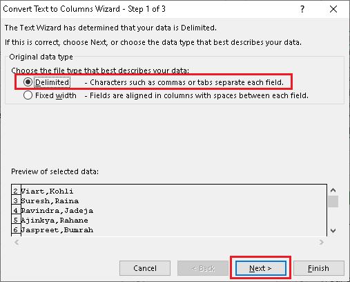
- After that, we will see the ‘Convert Text to Columns Wizard‘. In this screen, we must choose the file type describing the data of that corresponding file. We select the option ‘Delimited‘, which mainly allows us to separate the selected data at each specific character occurrence.
In our case, the comma character is the delimiter that separates the cell’s items. After selecting the ‘delimited’ option, we need to click on the ‘Next‘ button to move on to the next step.
- On the next screen, we must specify the specific type of delimiter from the Delimiters group. In our case, we select the ‘Comma‘ option and click the ‘Next‘ button. Also, we can see the Data preview, where each item is separated correctly.
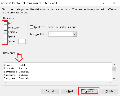
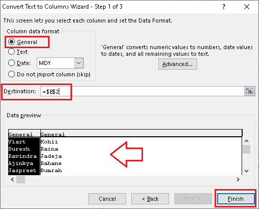
Depending on the availability of delimiters, we can also select multiple delimiters to split the data correctly or as desired. - Lastly, we must specify the data format for each column accordingly. Since we have text data in the cell, we must choose the ‘General‘ option or the ‘Text‘ option from the list. It is also the default formatting option. If the preview is displayed correctly after following all the previous steps, we must choose the destination cell. Next, we need to click on the ‘Finish‘ button.
After this, Excel will split the data accordingly.

Since we had one comma in the cell, so the data is separated into two columns. That is how splitting the cells works with the Text to Columns feature in Excel.
Split Cells in Excel Using Flash Fill
The flash fill feature is another handy way of splitting cells in Excel. However, this feature is only available in Excel 2013 and above. The flash fill method works by self-identifying the patterns and then applying corresponding patterns for all the consecutive cells. This method only works when we need to split the data into the connected cells.
Flash fill typically works in two ways:
- Background Execution by Excel
- Manually Triggered wherever needed
Background Execution by Excel
Excel automatically tries to find certain patterns in the background and then suggests users make the changes accordingly. Let us understand this with an example:
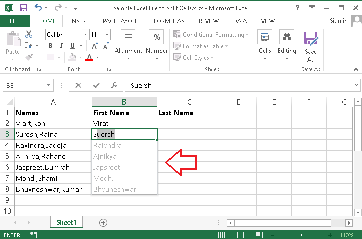
- With the original data on the left, we need to type the text element that we want to extract to the next column. Suppose we need to extract only the first names. Thus, we type the first name in the next column in the first row.

- Again, we type the first name in the next column in the second row. Now, we see that Excel automatically provides recommendations based on the last actions. We can press Tab or Enter key to accept all the recommendations and flash-fill the data.
- This way, we get the first names separated into the next column.

Similarly, we can extract the last names instead of first names.
Manually Triggered wherever needed
If Excel does not provide recommendations to split the data, we can manually trigger Flash fill in Excel. Let us now extract the last names using manual execution:
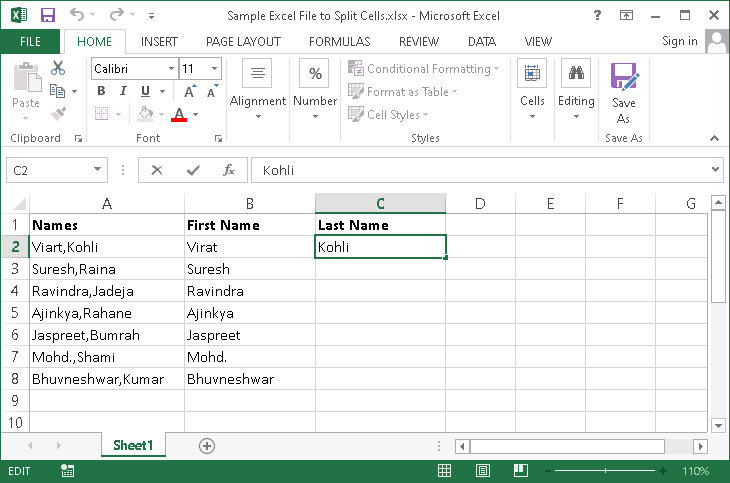
- We need to type the last name into any corresponding row with the original data on the left.
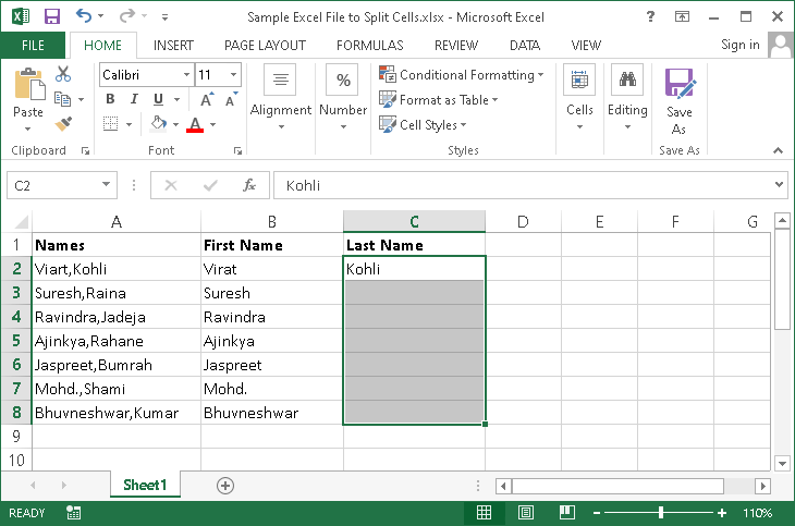
- Next, we need to select all the cells in the range that we want to fill. In our case, we select the entire column with the data on the left side (C2 to C8).
- After that, we must go to Home > Fill (drop-down) > Flash Fill. Alternately, we can press the shortcut ‘Ctrl + E‘ to perform the same task. This will automatically fill last names into the selected cells.
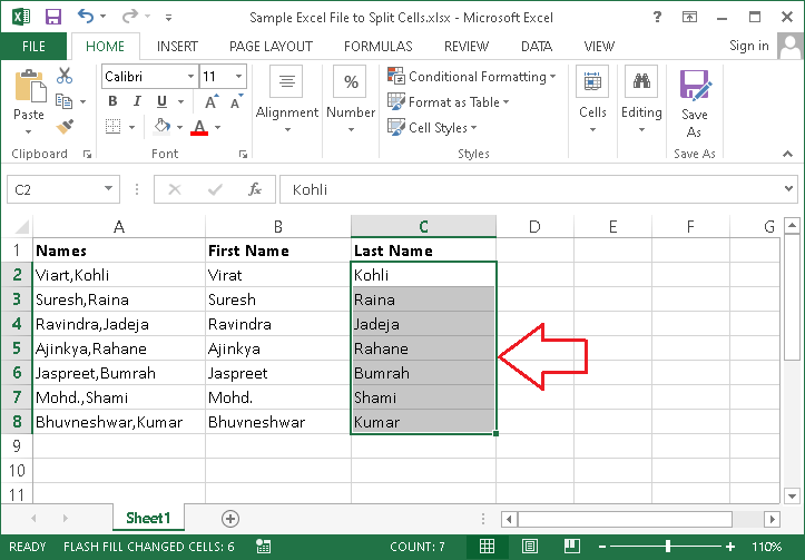
That is how we can split the cells in Excel using the Flash fill. We can try any of the Flash fill methods, such as the background or manual methods.
Split Cells in Excel Using Text Functions
The last and most efficient method to split cells in Excel includes the use of specific functions. This method is dynamic and works with any data. Although this method allows us to split data with certain rules applied to programs, we must have some advanced Excel skills. While the method is powerful, it is not just a point-and-click method. Instead, we need to efficiently think and apply proper functions with proper rules to split cells accordingly.
The following are the useful functions required for splitting Excel cells in many cases:
LEFT
This function returns the specified number of characters set from the beginning of the selected text string/ cell(s).
For example, suppose we use this function as:
We will get the result as:
WELC
Argument (4) tells the function only to return the initial four characters of the text string “WELCOME USER”.
RIGHT
This function returns the specified number of characters set from the selected text string/ cell(s) endpoint.
For example, suppose we use this function as:
We will get the result as:
USER
Argument (4) tells the function only to return the last four characters of the text string “WELCOME USER”.
MID
This function returns the specified number of characters from the middle of the selected text string/ cell(s). However, the starting position and length must be defined.
For example, suppose we use this function as:
We will get the result as:
COME
The second argument (initial 4) gives the function the nth character to start from, and the last argument (last 4) defines the length of the output string. Thus, the four characters starting at position four are “COME” in the string “WELCOME USER”.
LEN
This function only returns the total number of characters available in a selected text string/ cell(s).
For example, suppose we use this function as:
We will get the result as:
12
It is because the string “WELCOME USER” has a total of 12 characters, including space.
SEARCH
This function typically returns the total number of characters at which the specified character or text string is first found. The function reads the given string from the left character to the right and is not case-sensitive.
For example, suppose we use this function as:
We will get the result as:
8
The specified character (space) is initially located at the 8th position of the given string “WELCOME USER”. The last argument (1) is optional and is mainly used to tell the function where to start searching the specified character. Similarly, the FIND function is also used, but it is case-sensitive, unlike the SEARCH function.
SUBSTITUTE
This function typically replaces the specified characters with the newly defined characters in the selected text string/ cell(s).
For example, suppose we use this function as:
We will get the result as:
WELCOME DEAR
The last specified argument (1) defines which instance to replace. In the above example, only one instance exists, which is also the first instance. It is because the text characters “USE” are replaced with “DEA”. If we needed to replace more, we could change the number of arguments accordingly.
Let us now apply the necessary functions and rules with our example data:
We need to split the first names and the last names from the cells. For this, we need to use LEFT, RIGHT, SEARCH, and LEN functions in the following ways:
First Name
For the first names, we use the following function:
We will get the result as:

Where,
- The SEARCH function searches for the position of the space character in the string situated in the A2 cell. Then, it returns the total number of characters.
- Since we don’t require space characters in first and last names; thus, we subtract 1.
- The LEFT function then extracts the remaining characters from the left side.
Last Name
For the last names, we use the following function:
We will get the result as:

Where,
- The LEN function returns the length of the text string situated in the A2 cell.
- The SEARCH function returns the total number of characters at which the space character is first found in the string.
- Then, subtracting the LEN and SEARCH functions results in the number of characters left after the first located space character.
- The RIGHT function then extracts the remaining characters after the space character to the right.
After applying both the above functions in all the individual cells, we get the following results:

That is how we can split cells in Excel using the text functions.


