
Delete Data in Excel
Excel data is often brought into the worksheet from another source. Therefore, it contains many unwanted data that the user often requires to delete. Apart from this, we often encounter Excel rows and columns that are of no use, and therefore should be deleted from the Excel spreadsheet.
Excel offers two types of cell deletions, i.e., deleting the cell data and deleting the complete cell. The Delete operation could involve deleting a cell, any selected row or group of rows, a random column, and removing formatting in a cell selection.
This tutorial will briefly learn about the various methods to apply the Delete operation with their step-by-step implementations.
How to Delete the Data of any cell
- Select the cell(s) (by placing the cursor on the first cell and dragging till the last cell you want to delete) from which you want to delete the data. In the below example, we have selected a range of cells.
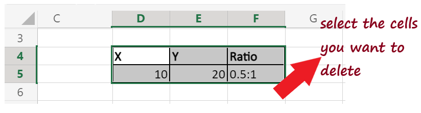
- Put your cursor on any of your selected cells and right-click on it. The following menu window will be displayed. Choose the Clear Content option, and all the data from the selected cells will be deleted.

- Instead of right-clicking, you can directly press the delete button on your keyboard, and it will also delete all the data of the selected cells.
- As shown below, all the data will be deleted.

NOTE: Remember, in the above option, we are not deleting any cell. We are only deleting the data or the content of that cell.
Clearing cell contents
So far, we have learned how to quickly delete or empty the cell content without removing the cell from the Excel worksheet. But if you notice it only deleted the content, the table behind the cells is still there in its output.
What if you want to clear or delete the content along with its formatting or cell comments. To get rid of this, Excel provides the Clear tool (located on the Home Tab). Using the clear drop-down menu, you can perform any of the following operations:

- Clear All: It removes all the data, formatting, comments present in the selected cell.
- Clear Formats: It only helps get rid of the selected cell’s formatting and leaves everything else intact.
- Clear Contents: It deletes only the data or the content of the selected cell(s). It works in the same way as pressing the Delete key.
- Clear Comments: It removes the comments in the cell selection without affecting anything else.
- Clear Hyperlinks: This clear option eliminates the active hyperlinks in the selected cell selection but leaves their cell entries as it is.
All the Drop-down options are very useful to quickly clear off the content, formatting, comments, and hyperlinks. Let’s have a look at the steps to implement clear cell contents to your Excel worksheet.
- Place your cursor and select the cell(s) from which you want to clear the content.

- Go to Home Tab -> Editing group -> Clear (it will be with eraser icon).

- The following options will appear as we want to delete the data to click on the Clear Contents.

- You will have the following output.

- You can see only the content is deleted; the comment and the formatting are still there. If you want to delete the content and the formatting, comments, and hyperlinks, you can choose the ‘Clear All’ option.
How to Delete a Row
- Click on the desired row number to select it.

- Right-click by placing your cursor on the row number of any of your selected cells. The following dialog window will appear. Click on the delete option.

- The entire row, along with all the data, will be deleted immediately, and the row beneath it will be shifted upwards.

Note: You can also delete multiple rows by selecting a single row first and then dragging your mouse cursor to select multiple rows. You can select non-contiguous rows by pressing the Ctrl key on your keyboard.
How to Delete a Column
- Click on the desired column alphabet to select it.
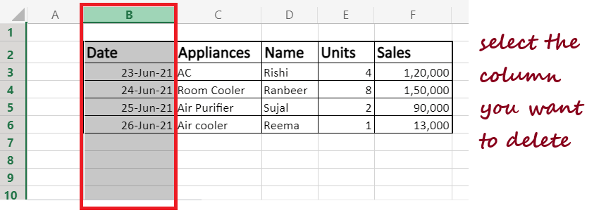
- Right-click by placing your cursor on the column alphabet of any of your selected cells. The following dialog window will appear. Click on the delete option.

- The entire column, along with all the data, will be deleted immediately, and the column towards its right will be shifted.

Note: You can also delete multiple columns by selecting a single column first and then dragging your mouse cursor horizontally left or right to select more columns. You can also select non-contiguous rows by pressing the Ctrl key on your keyboard.
Filter and delete Rows based on specific Value/Condition
Many times we need to delete rows or columns based on some specific values. It is usually required when we want to analyze some specific data. In this case, you need to filter out the data based on some specific condition and later delete the filtered data out from your Excel worksheet.
Excel supports inbuilt filter functionalities where the user can easily filter out their dataset on many criteria, unlike text, numbers, dates, colors, etc.,
We will briefly use different methods to filter out the data and later delete them.
Delete Rows that contain a specific text
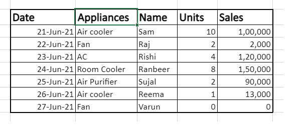
Suppose you have an Excel worksheet and you want to delete all the rows where the value of field appliances is ‘Fan’.
In that case, we will filter all the fields where the appliance’s value is Fan, and after filtering, we will delete all the filtered rows without touching the other rows.
Follow the below-given steps:
- Select any cell present in your dataset.
- Go to the Data tab. The following options will be displayed.

- Under the ‘Sort & Filter group, click on the Filter option (with a filter icon). This will result in putting the filters in all the headers’ cells.

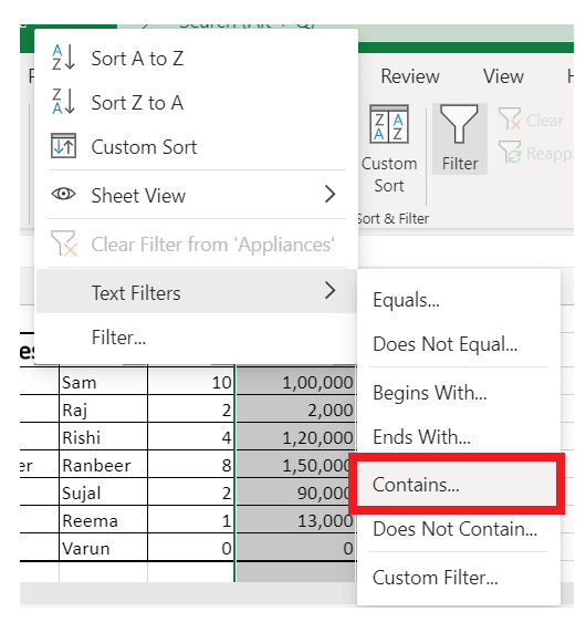
- Now, as we want to apply the filter in the Appliances, click on the Filter drop arrow (it resembles a downward-pointing triangle) in the Appliances header cell. You will have the following dialog box. Choose the ‘Text Filters’ option.

- The following drop-down will appear. Select the Contains option.
- The ‘Custom Filter’ dialog box will appear. In the Contain textbox type, ‘Fan’ and click on OK.

- As shown below, it will immediately filter all the row values and will display only the records where the appliance value is ‘Fan’.

- Now, as we have filtered the values, the next step is to delete them. Select the filtered values and place your cursor on any of the selected cells.

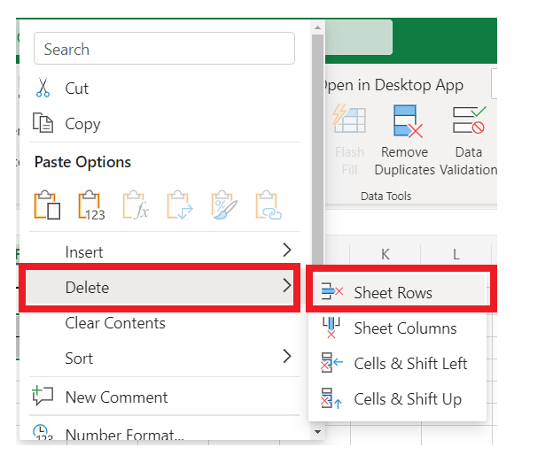
- Right-click on cells. A dialog box will appear. Click on Delete-> Sheet Rows.
- After deleting the rows, you will see no data in your sheet. To get back the data, we need to remove the filter. For that, click on the Data tab and click on the Filter icon.

- All the Rows which contain Fan as their appliance value will be deleted, and you will have the following output.

Filter and Delete Rows using Numeric Condition
The other option widely used to filter out numeric data is using a number condition (or a date condition).
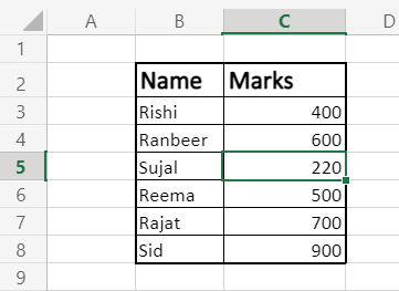
For example, let’s suppose we have extracted the data from an external source, and now we want to delete all the rows that have scored less than 300 in their exam.
Follow the below-given steps:
- Select any cell to apply the filter in the data.
- Go to the Data tab. The following options will be displayed.

- Under the ‘Sort & Filter group, click on the Filter option (with a filter icon). This will result in putting the filters in all the headers’ cells.

- Now, as we want to apply the filter in the marks, click on the Filter drop arrow (it resembles a downward-pointing triangle) in the Marks header cell. The following dialog box will appear. Choose the Number Filters option.

- It will further show all the number filter options. Click on the ‘Less than’ option.

- As soon as you click it, another dialog box will be displayed (as shown below). In the given field, enter the value ‘300’. Click on ok

- As shown below, it will filter out the records and show the dataset where mark values are less than 300.

- Select the filtered rows and place your cursor on any of the selected cells.

- Right-click on it. The following dialog box will appear. Click on the Delete Row option.

- After deleting the rows, you will see no data in your sheet. To get back the data, we need to remove the filter. For that, click on the Data tab and click on the Filter icon.

- As you can see, all the records below with value less than 300 has been deleted, and you have your filtered output.


