Advanced Formulas in Excel

Microsoft Office Excel is the most popular and famous tool. It helps small, medium, and large-scale businesses to maintain, store, and analyze data into useful information with its qualities to execute functions and advanced excel formulas.

95% of the Excel users apply the basic form. There are functions and advanced excel formulas that are used for complex calculations. The functions are designed for easy lookup and formatting of a large pool of data, whereas the advanced excel formula is implemented to get new information from a given particular set of data.

All advanced excel formulas can transform lengthy manual tasks into a few seconds of work. Below are some advanced formulas like VLOOKUP, INDEX, MATCH, IF, SUMPRODUCT, AVERAGE, SUBTOTAL, OFFSET, LOOKUP, ROUND, COUNT, SUMIFS, ARRAY, FIND, TEXT, and many more.

1. INDEX MATCH

This is an advanced alternative to the VLOOKUP or HLOOKUP formulas which have several drawbacks and limitations. INDEX MATCH is a powerful combination of Excel formulas that will take your financial analysis and financial modeling to the next level.

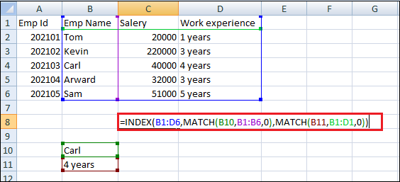
• INDEX returns the value of a cell in a table based on the column and row number.
• MATCH returns the position of a cell in a row or column.

Here is an example of the INDEX and MATCH formulas combined. In this example, we look up and return years of work experience of employees based on their names. Since name and year are both variables in the formula, we can change both of them.

2. IF combined with AND / OR

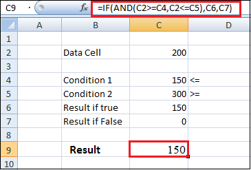
Who’s spent most of the time doing various types of financial models faced nested IF formulas can be very difficult. Combining IF with the AND or the OR function can be a good way to keep formulas easier to audit and easier for other users to understand

In the example below, you will see how to use the individual functions in combination to create a more advanced formula.

3. OFFSET combined with SUM or AVERAGE

The OFFSET function on its own is not particularly advanced, but when we combine it with other functions like SUM or AVERAGE, we can create a pretty sophisticated formula.

Suppose you want to create a dynamic function that can sum a variable number of cells. With the regular SUM formula, you are limited to a static calculation, but you can have the cell reference move around by adding OFFSET.

4. CHOOSE

This advanced excel formula removes lengthier IF function statements and pulls the particular set of data you want. It is used when there are more than two outcomes for a particular given condition.

The CHOOSE function is great for scenario analysis in financial modeling. It allows you to pick between a specific number of options and return the “choice” you’ve selected.

5. XNPV and XIRR

Suppose you’re an analyst working in investment banking, equity research, financial planning & analysis (FP&A), or any other area of corporate finance that requires discounting cash flows. In that case, these formulas are a better option.

Simply put, XNPV and XIRR allow you to apply specific dates to each cash flow that’s being discounted. The basic problem with Excel NPV and IRR formulas is that they assume the periods between cash flow are equal. Routinely, as an analyst, you’ll have situations where cash flows are not timed evenly, and this formula is how you fix that.

6. SUMIF and COUNTIF

These two advanced formulas are great uses of conditional functions. SUMIF adds all cells that meet certain criteria, and COUNTIF counts all cells that meet certain criteria.

7. PMT and IPMT

If you work in commercial banking, real estate, FP&A, or any financial analyst position that deals with debt schedules, these two formulas will be very helpful for you.

The PMT formula gives you the value of equal payments over the life of a loan. You can use it in conjunction with IPMT, which tells you the interest payments for the same type of loan, then separate principal and interest payments.

8. LEN and TRIM

LEN and TRIM formulas are useful for financial analysts who need to organize and manipulate large amounts of data. Unfortunately, the data we get is not always perfectly organized, and sometimes, there can be issues like extra spaces at the beginning or end of cells.

The LEN formula returns a given text string as the number of characters, which is useful when you want to count how many characters there are in some text.

The TRIM formula is used to trim or remove extra spaces which appear when a set of data is copied from another source.

9. CONCATENATE

Concatenate is not a function on its own. It’s just an innovative way of joining information from different cells and making worksheets more dynamic.

This function combines both LEFT and RIGHT Functions in Excel, where a new column of data is prepared by setting the variable to pull a particular section of the data from left and right. This is a very powerful tool for financial analysts performing financial modeling.

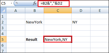
In the below example, you can see how the text “New York” plus “, is joined with “NY” to create “New York, NY. This allows you to create dynamic headers and labels in worksheets. Now, instead of updating cell B8 directly, you can update cells B2 and D2 independently. With a large data set, this is a valuable skill to have at your disposal.

10. CELL, LEFT, MID, and RIGHT functions

These advanced Excel functions can be combined to create some very advanced and complex formulas to use. The CELL function can return a variety of information about the contents of a cell, such as its name, location, row, column, and more.

• The LEFT function can return text from the beginning of a cell (left to right).
• MID returns the text from any start point of the cell (left to right).
• And RIGHT returns the text from the end of the cell (right to left).

11. RANDBETWEEN()

This advanced excel formula is used to generate a random number between the values you have set. It helps when you want to simulate some results or behavior in the spreadsheets.

12. PROPER Function

This proper function is used to capitalize or uppercase the letters of a sentence in the cells. It can be done in a customized way. You can selectively change the letters in whatever format you want.

13. ROUND Function

This function is used to round up data with many digits after the decimal point for the convenience of calculation. You do not need to format the cell.

14. VLOOKUP

The function is used to look up a piece of information in a large segment of data and pull that data to your newly formed table. You have to visit the function option. The insert function tab will let you enter ‘VLOOKUP’, or you can find it in the list. Once it is selected, a wizard box will open with a different set of box options. You can enter your variables into:

• Lookup_value: This is the option where your typed variables will go to look for the values in the cells of the larger table for information.
• Table Array: It sets the range of the large table from where the information will be drawn. It sets the extent of the data you want to pick.
• Col_index_num: This command box specifies the column from where data has to be pulled.
• Range_lookup: Here, you enter either true or false. The true option will give the information set closest to what you want to find when anything does not match the variables. When you enter false, it will give you the exact value you are looking for or show #N/A when the data is not found.

15. Unit conversion by CONVERT()

The CONVERT() advanced excel formula helps to determine the converted value of data in different units. The versatile function can also be used to convert currencies and many other things.

---