
VLOOKUP Errors in Excel
MS Excel, short for Microsoft Excel, is a powerful spreadsheet program that enables users to record data and perform various operations using functions and formulas within multiple cells. VLOOKUP is one of the existing Excel functions. This allows us to search for and return data from any other column in our entire workbook. However, the function can seem tricky if we’re not familiar with it, especially when using it directly in a cell. If we apply the VLOOKUP function incorrectly, it gives various errors or may give wrong results.

This article discusses the various VLOOKUP errors that we commonly encounter while working in Excel. Due to VLOOKUP errors, we get either incorrect results or specific error codes that indicate that something is wrong with the formula applied.
What are the common VLOOKUP Errors in Excel?
In Excel, VLOOKUP is a widely used function that helps extract specific values from various data sources. However, the function also has several limitations. When we do not follow certain limitations or specifications of VLOOKUP, it usually leads to unexpected results and errors. This is why many Excel experts consider VLOOKUP to be one of the most complex Excel functions.
The following are the most common errors that often appear while using the VLOOKUP function in Excel:
- VLOOKUP #N/A Error
- VLOOKUP #NAME? Error
- VLOOKUP #REF! Error
- VLOOKUP #VALUE! Error
To avoid VLOOKUP errors, we must ensure to use properly formatted data without the blank cells, incorrectly formatted values, and deleted formulas. Also, we can use the IFERROR function with VLOOKUP. It helps to ignore the error and return whatever is placed in the place of the error.
Let us now discuss each VLOOKUP error in detail and know the ways to fix it accordingly:
#N/A Error in VLOOKUP
The #N/A error in VLOOKUP usually occurs when the formula does not find the desired lookup value to produce results. The term N/A means ‘Not Available’. This error can occur due to one of the following reasons:
1. The lookup value is misspelled
led
We may type a lookup value with some spelling mistakes when dealing with a large data set. In that case, the VLOOKUP formula returns the #N/A error because it does not find the mistyped value in the defined table range.
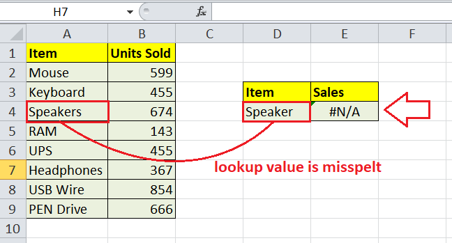
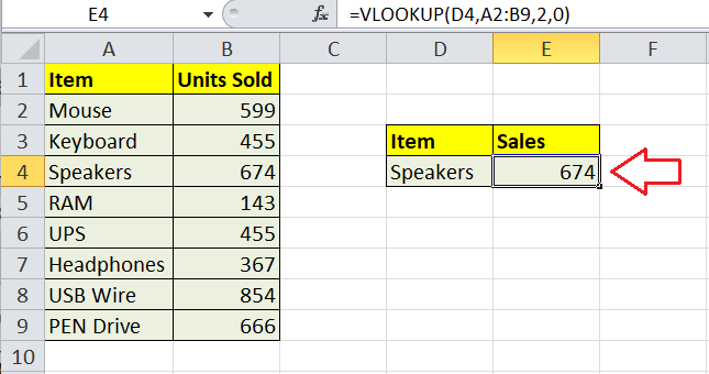
In the above sheet, the formula searches for a value ‘Speaker’ while the table range has a value entered as ‘Speakers’. The formula does not find the exact match as one ‘s’ is missing in the lookup value. Correcting the typo in the lookup value fixes the #N/A error.
2. #N/A error in exact match VLOOKUP
When we apply the VLOOKUP to search for an exact match (range_lookup argument is FALSE), the formula returns the #N/A error if no exact match is found in the defined table range.

In the above sheet, the formula is searching for an ID with the number 100 (in cell D4) returns an #N/A error because the minimum ID number in the range is 101. The formula does not find the exact match. Giving the proper matched lookup value fixes the #N/A error.

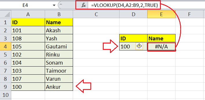
3. #N/A error in approximate match VLOOKUP
When we apply the VLOOKUP to search for the closest or approximate match (range_lookup argument is TRUE), the formula returns the #N/A error in the following two cases:
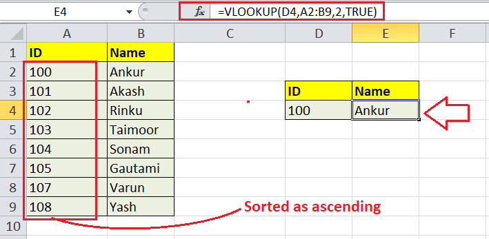
- The value column in a defined table (lookup array) is not sorted as ascending.
In the above sheet, the order of recorded IDs is mixed up. Despite a value of 100 existing in the defined range, the formula cannot lookup for a value with the range_lookup argument set to TRUE, causing the #N/A error. It is because column A or IDs are sorted in ascending order. Sorting the range column as ascending fixes the #N/A error.
- The lookup/ search value is smaller than the lowest value written in the range.

The formula returns the #N/A error in the above sheet while looking for the number 100 (in cell D4), even if it is set to look for an approximate result. The reason for this error in the above sheet is the smaller value (100) than the lowest value (101) in the range. We must not look for smaller values when using approximate match VLOOKUP. However, the formula works perfectly when the lookup value is greater than the defined value in the range.
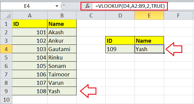
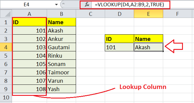
4. The lookup column is not the left-most column
One of the most common reasons for the #N/A error in VLOOKUP is that it is given a table array or a range that does not contain the lookup column to the left. The LOOKUP formula cannot return a value from its left. Therefore, a lookup column must always be structured to the left-most side in the table array. We usually forget this limitation of the VLOOKUP formula and get the respective error.
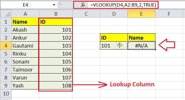
Moving the lookup column to the left-most side in the defined table array fixes the #N/A error. After moving the column to the left-most side, we must specify the array table or a range again.
If it is not possible to switch the columns or reorganize data to make the lookup column the left-most column due to some reasons, we must avoid using the VLOOKUP formula. Instead, we can use INDEX and MATCH functions together as an alternative to the VLOOKUP.
5. Numerical values formatted as text
The formatting of cells also plays an important role in VLOOKUP. If our data set contains numbers formatted as text, either in the main or lookup table, the VLOOKUP formula will usually return a #N/A error. This usually happens when we copy or import data from other sources instead of entering it manually. Also, the numbers starting with an apostrophe are interpreted as text by Excel.
If our sheet has text-formatted numbers, the error indicator is displayed for such cells. If we select such cell(s), Excel also displays a message accordingly.

Converting the text-formatted numbers to numbers usually fixes the #N/A error. To convert numbers that are stored as text into exact numbers, we must first select all such problematic cells/numbers. After that, we need to click the error icon and select the ‘Convert to Number’ option from the list.

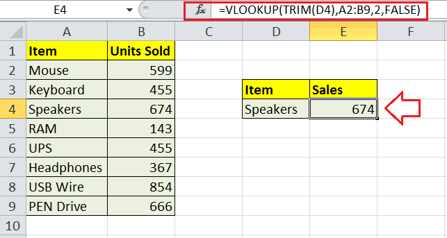
6. Leading or trailing spaces
Another common reason behind the #N/A error in VLOOKUP is the presence of one or more extra spaces, either in the beginning or the ending of the cell value. There can be the following two cases when dealing with spaces in VLOOKUP:
- Extra Spaces in the lookup value: If the cell used for the lookup value contains an extra space before and/or after the value, the VLOOKUP formula returns the #N/A error.

If our sheet has many cells with extra spaces, we can use the TRIM function and wrap the lookup value inside it to get the desired result by VLOOKUP.
- Extra spaces in the lookup column: If one of the cells or the entire lookup column contains an extra space before and/or after the value, the VLOOKUP formula returns the #N/A error.

In this case, it is not easy to fix the error in VLOOKUP. We have to edit each respective cell and delete the spaces. However, if there are way too many cells with spaces in the lookup column, it is better to use a combination of INDEX, MATCH, and TRIM functions as an array formula in the following way:

It is essential to note that after typing the entire formula, we must press ‘Ctrl + Shift + Enter’ instead of only the Enter key. It is required because we are using an array formula.
#NAME? Error in VLOOKUP
#NAME? error is one of the most common and easy to fix VLOOKUP error. This error typically appears when we accidentally enter the wrong or misspelled function name. For example, we may type VLOKUP or CLOOKUP in place of the VLOOKUP and see the #NAME? error instead of the expected results.

In the case of the misspelled function name, Excel does not find the function in the library and returns the values as #NAME? error type.
To fix the #NAME? error in VLOOKUP, we must ensure to enter the correct function or formula name. After the function name is corrected, the error is resolved.

#REF! Error in VLOOKUP
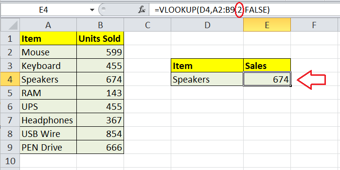
The #REF! error in VLOOKUP appears because of the wrong reference number. When we enter the VLOOKUP formula, we must specify the exact column index number; a column used to obtain a result. If we accidently type the column index number higher than the selected range, the VLOOKUP formula will return the #REF! error.
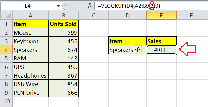
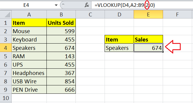
We have supplied the correct table range and the lookup value in the above sheet, but the entered column index number (which is 3) is out of the selection range. Since we have selected the range A2:B9, only two columns are supplied within the table range. Correcting the column index number fixes the #REF! error in VLOOKUP.
Since we have only two columns and column second is the main column we need to extract the resultant value from, we specify the column index number as 2, not 3.
#VALUE! Error in VLOOKUP
Generally, the #VALUE! error in VLOOKUP occurs when a value supplied in the respective formula is of a wrong data type. In addition to this, there are some other reasons as below:
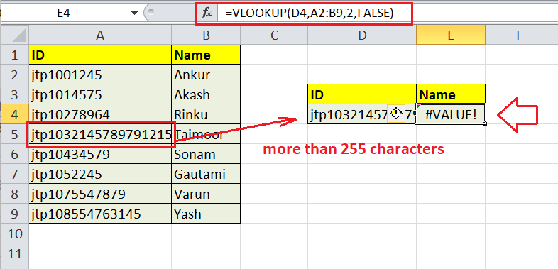
1. Lookup value contains more than 255 characters
Unfortunately, Excel’s VLOOKUP formula cannot look up values exceeding 255 characters. If there are more than 255 characters in the Lookup value, the formula returns the #VALUE! error.
To fix #VALUE! errors in such cases, we must use a combination of INDEX, MATCH functions in the following way:
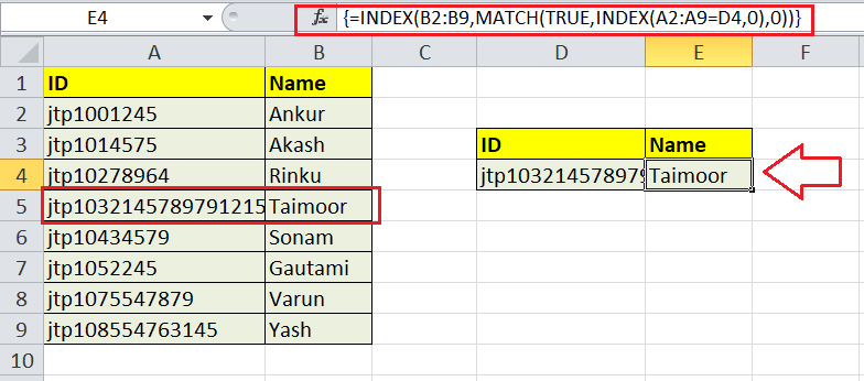
After entering the entire INDEX and MATCH combination formula, we must ensure to press ‘Ctrl + Shift + Enter’ instead of only the Enter key.
2. Missing Parameters or Arguments
If the VLOOKUP formula is applied with any missing argument, it can lead to #VALUE! error. The VLOOKUP formula must be supplied with the LOOKUP value, then the table range, followed by a column index number and match type.
In the following sheet, the #VALUE! error appears due to a missing LOOKUP value in the applied formula.

To fix the #VALUE! error in VLOOKUP, we must supply all the necessary parameters and ensure they are in proper order.
3. The col_index_num is less than 1
If we accidently type the column index number less than 1, the VLOOKUP formula will return the #VALUE! error.

In the above sheet, we have supplied the correct table range and the lookup value, but the entered column index number (which is 0) is less than 1. It is unusual that a user intentionally types a column number below 1 because we use VLOOKUP to obtain results from a specific column. That means there must be at least a column within the sheet. However, there may be cases when a number is less than 1, especially when this argument is returned by some other function nested in our VLOOKUP formula.
Correcting the column index number fixes the #VALUE! error in VLOOKUP.
Avoiding the VLOOKUP Errors
Excel’s VLOOKUP function has several limitations, more than any other existing function in Excel. Because of such limitations, we must always use this function from the Insert Function Wizard. Using the wizard, we get information about the desired arguments, which helps to eliminate errors. In addition, we can follow the precautions below to avoid or prevent errors in our sheets with VLOOKUP:
- A data range has duplicate values: The VLOOKUP function cannot provide the exact result when we have duplicate values in our data range. The function only displays the results from the first value it finds, leaving all other duplicate values intact. Thus, VLOOKUP cannot be used for data ranges with duplicate values.
- Trying to extract data from the left: It is essential to note that the VLOOKUP function does not work to look up the data to its left. When we apply the VLOOKUP and enter or supply data range, we must ensure that the search column is at the furthest left column in our defined data range.
- VLOOKUP is case-insensitive: Excel’s VLOOKUP function is case-insensitive. This means that the function treats uppercase and lowercase letters as the same characters. If our sheet has both upper and lowercase letter entries, the VLOOKUP function will work accordingly for both cases.
- A column is inserted or deleted in a table: After inserting the VLOOKUP formula, we must avoid changing a data set. If we make changes like adding or deleting a column, the VLOOKUP function may cause unexpected errors. When we add or delete a column, the arguments like col_index_num and table_array get changed in the dataset and the VlOOKUP function. This further causes the VLOOKUP errors.
- Copying a formula with relative reference: We must avoid copying the VOOLUP formula, especially when we have relative references. If we need to copy formulas, we can use absolute cell references. We need to include the $ sign in the table_array to make cells absolute. We can press the F4 function key to make the cell(s) absolute immediately. By making cells absolute, we tightly lock their references, and copying them into another cell no longer creates a problem.


