Text Wrapping in Excel

MS Excel or Microsoft Excel is the widely popular and most useful spreadsheet software developed by Microsoft. It enables users to enter data into tables formed by the intersection of rows and columns. Also, each Excel workbook consists of multiple sheets or worksheets. Numbers, text, and symbols are the most common data types used in Excel. While recording text data or strings, we sometimes notice that the sentence keeps overlapping on other Excel cells. This usually happens when recording long text data such as long sentences or paragraphs in an Excel cell. Text wrapping is a built-in feature of Excel to overcome this problem.

This article discusses various step-by-step methods to apply text wrapping in Excel to desired cells within a sheet. The article also discusses some common ways to remove text wrapping when needed. Before moving on to the methods, let’s first take a brief introduction to the wrap text feature of Excel.

What is the wrap text feature in Excel?

Wrap text is a built-in Excel feature that enables users to display long text strings of an Excel cell in multiple lines without changing the width. However, we can manually change the width of the cell if required. Wrap text is a part of Excel formatting settings and changes the view only, not the values of text strings. This feature is primarily used for cells where text strings exceed the size of the cell width and overlap on other adjacent cells.

The main reason for using the wrap text feature is that lengthy text strings in a cell become visible even if the next adjacent cell contains content. By default, if we enter a long text string in concurrent adjacent cells, the content will not be displayed entirely within the cells. To view the contents of a specific cell, we have to select the cell and read it from the formula bar. By wrapping the text, we make the text strings visible within the width of the same cell without allowing them to overflow onto other cells. It uses the increased cell height to fit the content in the cell. This special formatting feature enhances the readability of worksheet data.

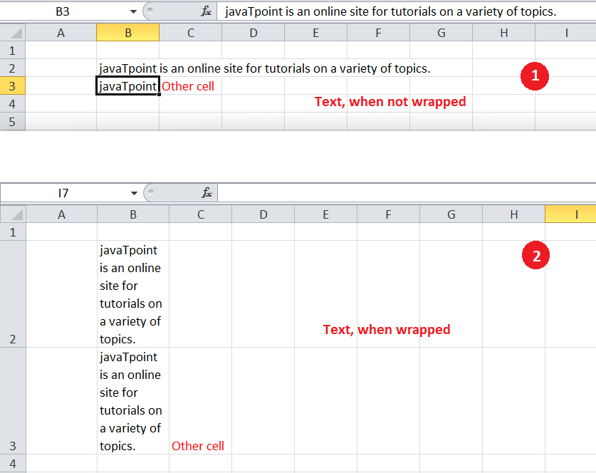
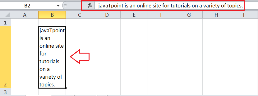
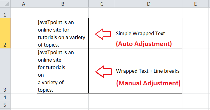
The following image displays how the text looks like before (1) and after (2) wrapping:

How to add/ insert Text Wrap in Excel?

Excel usually provides several ways to perform a specific task. Similarly, when wrapping text in Excel, there are multiple options. Some options are fast, while others are relatively slow. The following are some of the most common ways or methods to insert text wrap in one or more desired cells:

• Wrap Text using the Ribbon
• Wrap Text using the Format Cells
• Wrap Text using the Keyboard Shortcut
• Wrap Text using the Quick Access Toolbar
• Wrap Text using the Adjustment of Row Height and Column Width
• Wrap Text using the Line Breaks

The above four methods usually wrap text automatically, while the fifth method wraps text automatically and manually. Furthermore, the last method helps users wrap text in desired cells manually. In the last method, we usually add line breaks at fixed positions, which serve as an alternative to the wrap text feature.

Let us discuss each method in detail:

Method 1: Text wrapping using the Ribbon

Excel ribbon provides shortcuts for built-in commands and tools using which we can perform almost all the tasks. Also, we can add/ remove additional tools accordingly. The Ribbon also contains necessary options to wrap text within the desired Excel cells in the worksheet.

Suppose we have the following example sheet where cell B2 has a lengthy sentence, and we need to wrap the contents of this cell.

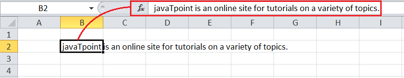
Since the text string (sentence) is going to multiple columns, it will not be entirely displayed if other consecutive cells also have contents. The following are the steps to wrap text in cell B2 by using the Excel ribbon:

• First, we need to select the cell that we want to wrap. In our case, we select cell B2.
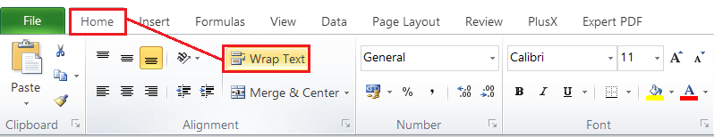
• Next, we need to navigate the Home tab and click the ‘Wrap Text’ button under the ‘Alignment’ section. This Wrap Text button acts as a toggle button and can be turned on/off to wrap and unwrap the text accordingly.
  
• As soon as we click the Wrap Text button, the text in the selected cell is displayed or divided across multiple lines without going to other cells.
  
  In the above image, we can see that the column width is still the same while the row’s height is adjusted to fit the contents in the cell.

Similarly, if we have multiple cells where we need to wrap text, we must select all those cells and click the ‘Wrap Text’ button once. We can select all the desired contiguous and non-contiguous Excel cells as required.

Method 2: Text wrapping using the Format Cells

The traditional method of wrapping text in an Excel cell involves using the Format Cells dialogue box. The Format Cells dialogue box provides a variety of multiple number formats using which we can set preferences for cell formatting, including wrapping text where desired.

Let us again consider the previous example with a long text in cell B2 where the text string gets rolled on other cells like C2, D2, E3, etc. To warp text in the cell B2 using the Format Cells, we must perform the following steps:

• First, we need to select one or more cells where we wish to wrap text. Like the previous method, we select cell B2.
• After selecting the effective cell (or cells), we need to launch the Format Cells dialogue box. We must press the right-click button via the mouse and click the ‘Format Cells’ option.
  
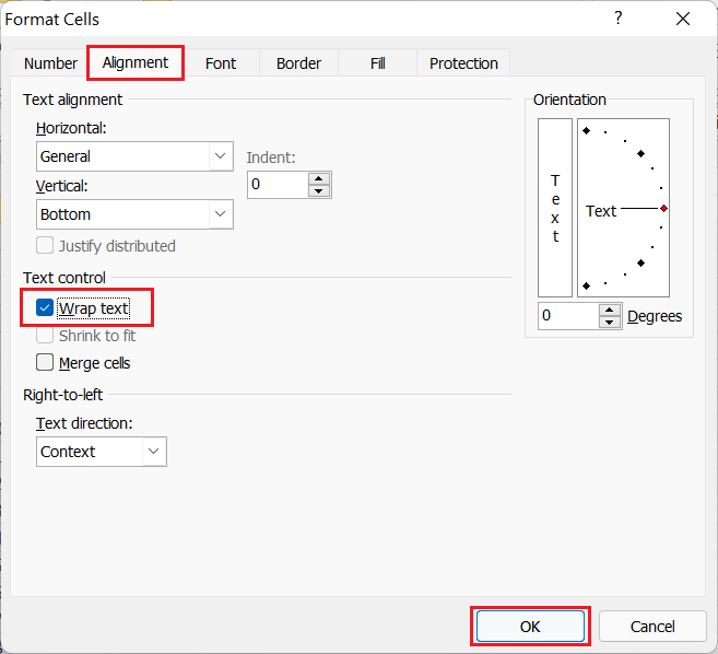
  This will open the Format Cells dialogue box, as shown below:
  
  We can also open the Format Cells dialogue box instantly by using the keyboard shortcut ‘Ctrl + 1’, where the key ‘1’ needs to be pressed from the keyboard area. If we press the key ‘1’ from the numeric pad of the keyboard, the shortcut does not work as expected.
• We need to go to the Alignment tab in the dialogue box and select the check box associated with the Wrap Text option under the category Text Control. After selecting the checkbox, we must click the OK button to apply the changes.
  
  In the below image, we can see that the text in cell B2 is wrapped accordingly.
  

The above steps also work for wrapping text in multiple cells within the sheet. We only need to select the corresponding cells before using the Format Cells dialogue box.

Method 3: Text wrapping using the Keyboard Shortcut

Excel provides a wide range of built-in keyboard shortcuts that help perform specific operations with ease. It has a unique shortcut key combination for almost all common functions. If no keyboard shortcut is available for a specific task, Excel allows users to create their own customized keyboard shortcuts. Also, if the associated command or tool is present on the Excel ribbon, the Alt key shortcut method works perfectly.

Unfortunately, there is no predefined keyboard shortcut key combination when we need to use Wrap Text Tool in Excel. However, we can take advantage of the Alt key method. According to this method, we must first press the Alt key on the keyboard during the Excel Active Window Mode. This usually enables certain key characters on the Ribbon, and each key character is associated with a particular tool or command. Since we need to apply text wrap, we must press the H key and the W key. We don’t need to press the keys simultaneously. Instead, we must press each key one by one, e.g., Alt, H, W (or we can say: Alt + H + W).

Steps to wrap text in excel by using the keyboard shortcut

• Like other methods, we need to select the desired cells to be wrapped.
• After selecting the cells, we must press the shortcut keys “Alt + H + W”. As discussed above, we must press one key in a sequence.
• After the last key (W) is pressed, the Wrap Text feature comes into action and wrap text in all the selected cells at once.

Method 4: Text wrapping using the Quick Access Toolbar

Like keyboard shortcuts, another quick way is to use the Quick Access Toolbar to access any tool or command in Excel. But, before we can start using any specific tool, we need to add it to the Quick Access Toolbar. Once added, we can use the respective feature as many times as required in all excel files/ windows.

The following are the steps to add or insert the Wrap Text Tool on Excel’s Quick Access Toolbar and use it accordingly to apply text wrapping to the desired cell (s):

• First, we need to navigate the Home tab and locate the ‘Wrap Text’ button under the category Alignment. We need to press the right-click mouse button on the Wrap Text button.
  
• After pressing the right-click button, we will see a list of a few options. We must click the option ‘Add to Quick Access Toolbar’ from the list.
  
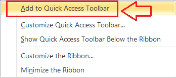
  This will instantly add a shortcut for the Wrap Text command on the quick access toolbar. The shortcut will look like this:
  
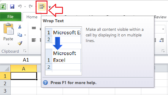
  After the ‘Wrap Text’ shortcut has been added, we only need to click it once to apply text wrapping. However, we must select all the cells before clicking on the shortcut.

Method 5: Text wrapping using the Adjustment of Row Height and Column Width

As seen in the above methods, long text strings are wrapped in the cell by adjusting the cell’s height. Therefore, we can directly adjust the height of the specific cell accordingly to make the cell content fit within the width. The desired cells height can be adjusted manually as well as automatically.

To manually adjust the height of a specific cell or row, we need to click and drag the border from the respective row header. If we manually adjust the height, it will become difficult when we need to do this for multiple cells.

Using automatic row height adjustment will reduce our workload, and we can easily adjust the height of multiple cells or rows at once. To auto-adjust the height, we can perform the following steps:

• First, we have to select all the desired cells to wrap.
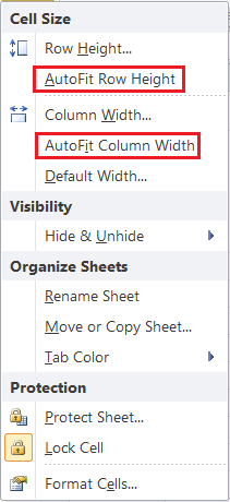
• Next, we need to navigate to the Home tab and select the Format option under the category Cells, as shown below:
  
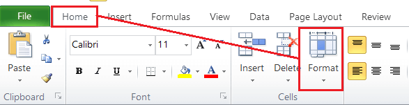
• After that, we have to select AutoFit Row Height option from the list. If we don’t have very long text strings, we can also try adjusting the cell’s width by clicking the Autofit Column Width option.
  
  It will automatically wrap the text in all the selected cells by adjusting the height and width we selected.

Method 6: Text wrapping using the Line Breaks

We can break any long text string into multiple parts to fit in a specific cell width using line breaks. We can manually choose the point where we want the text to start in a new line within the cell. To put a breakpoint in text strings in the desired cell, we should follow below steps:

• First, we must double-click on the cell where we need to insert a line break. This will open Cell Edit mode. Alternately, we can also select the cell and press the F2 function key on the keyboard.
• Once the cursor starts blinking within the selected cell, we must move and place the cursor to the specific point of the text string where we wish to break a line. It is better to click at the desired point using the mouse while in the cell edit mode. The formula bar also allows editing the cell contents.
• After placing the cursor at the desired point within the text string, we must click the Alt key and the Enter key simultaneously, i.e., ‘Alt + Enter’.

How to remove/ delete Text Wrap in Excel?

When we need to remove text wrap from a cell, we must follow the same steps we used while inserting text wrap. This means we can click on the Wrap Text button from Ribbon to insert text wrapping and remove inserted text wrapping. Similarly, we can also use the keyboard shortcut ‘Alt + H + W’ to insert/undo text wrapping. We must ensure that the desired Excel cell (s) is selected before undoing the text wrapping.

Important Points to Remember

• We can quickly select contiguous and non-contiguous cells when wrapping text in multiple Excel cells as desired. We only need to click on the first and last cells of the specific range while holding down the Shift key on the keyboard for selecting contiguous cells. For non-contiguous cells, we need to click on each respective cell in the sheet while holding down the Ctrl key.
• Some specific spelling or words may break across two lines when wrapping text in an Excel cell. It typically happens when the corresponding cells contain lengthy words. In such cases, we must adjust the width of the column by dragging the column header’s left-right lines.