Strikethrough in Excel
First of all, it is important to understand that what is strikethrough and why it needs. Strikethrough is a type of formatting option in Excel. But now you are thinking that what does it mean. Basically, strikethrough refers to drawing a line through a value in the Excel cells.
In this chapter, we are going to learn about strikethrough, features, advantages of using it and its examples. We will discuss the given topic below –
- What is strikethrough
- Features of strikethrough
- Excel does not have strikethrough option
- Apply strikethrough on Excel data
- Shortcut key to apply strikethrough
- Add strikethrough option in Quick Access Toolbar
- Strikethrough Examples
- Example 1: Strikethrough with conditional formatting
What is strikethrough?
As we described that the strikethrough is a type of formatting option to draw a line through a value in Excel. Strikethrough cross something by drawing a line through it. Now, let’s understand with an example.
Strikethrough is a text formatting method that you can apply to Excel data. It usually applies to the text stored in Excel cells. You can use strikethrough on a single Excel cell data or a range of cells.
Text with strikethrough is a cut text. This text looks like this, as shown in the below screenshot –
Features of strikethrough
Know the following features about strikethrough in MS Excel –
- Strikethrough can be applied on any type of data, such as text, number, date, etc.
- It is a formatting feature that is not directly available in MS Excel.
Excel does not have strikethrough option
Those who worked with MS Word know that MS Word has an option Strikethrough in the Home tab of MS Word ribbon while MS Excel does not have such option. There is no option to strikethrough the text in Excel.

So, the big question is that how can we apply strikethrough in Excel.
In this chapter, we will go through several other methods to apply as well as remove strikethrough in MS Excel.
Apply strikethrough on Excel data
There is a long way to apply the strikethrough on Excel data as it is not directly available in Excel like MS Word. But you can apply it by following few simple steps. We have taken some data in an Excel worksheet on which we will apply the strikethrough formatting.
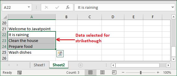
Step 1: Select the data in the given dataset on which you like to apply strikethrough.
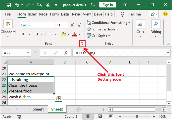
Step 2: In the Home tab, go to the Font section and click on the small down arrow icon (Font Setting button) present in its bottom right corner.
Step 3: A Format Cell panel will open, where mark the Strikethrough option and click OK.

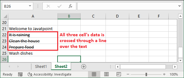
Step 4: Now, you see that all three selected data is crossed through by a line over it.
Each time you have to follow the same steps if you want to apply strikethrough.
Shortcut key to apply strikethrough
Excel does not have the strikethrough option but has a shortcut key to apply the strikethrough on the text stored in Excel cell. The strikethrough shortcut key is –
You just have to select the data on which you want to apply the strikethrough formatting.
Press this shortcut key to apply the strikethrough on the selected Excel data automatically.
Tip: If you want to apply the strikethrough text formatting on multiple cells data. Select that range of cells and then apply strikethrough using the Ctrl+5 shortcut key.
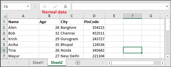
Data before applying Strikethrough
See, we have some data stored in an Excel worksheet that is currently normal without applying strikethrough formatting.
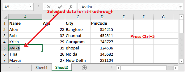
Select a cell or range of cells and press the Ctrl+5 shortcut key to apply strikethrough on the selected data range. For example, we have selected A5 cell.
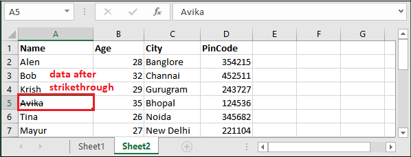
Date after applying strikethrough
Now, we have applied strikethrough formatting on column A (a range of cells) and you will see that a line crossed through the data over it.
Data with strikethrough looks like this –
Similarly, you can apply strikethrough on numeric data.
Add Strikethrough option in Quick Access Toolbar
Every time you don’t remember the shortcut key, that is are rarely needed. So, it is best to add the strikethrough option (icon) in Excel Quick Access Toolbar (QAT). Next time, whenever you need you can directly use it from there.
We have some steps for it –
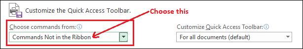
Step 1: Click on the small icon in Quick Access Toolbar and then click the More Commands in the list.

Step 2: A panel will open where choose Commands not in Ribbon in Choose command from field.
Step 3: Scroll down the list, select Strikethrough command and click the Add button to move it to Excel ribbon.
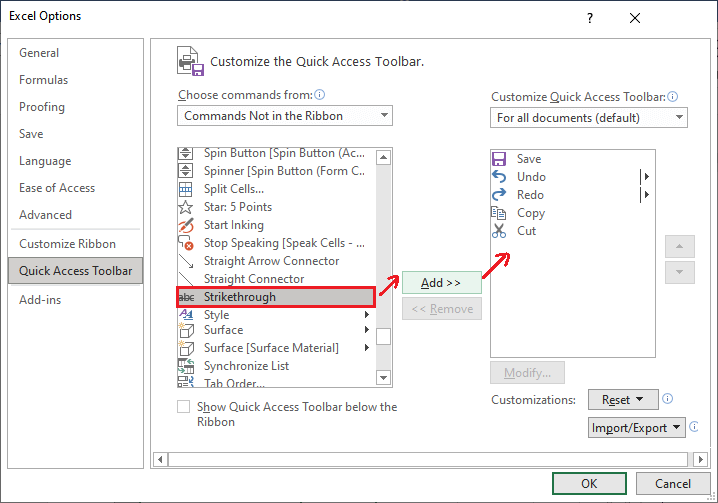
Step 4: When the Strikethrough option is moved to the right side list, click the OK button to save the changes.

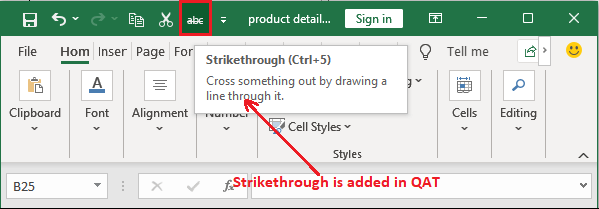
Step 5: See that the Strikethrough option is added in Quick Access Toolbar. Now, you can directly perform strikethrough action from here.
Strikethrough Examples
Till now, we have explained the strikethrough and how to apply it on Excel cells data. Now, take an example of strikethrough. It can be used to show the complete task in Excel. We will show you an example of conditional formatting with strikethrough.
Example 1: Strikethrough with conditional formatting
In this example, we will use conditional formatting to strikethrough the cell data like the color formatting. For this, let’s take a scenario first.
Scenario
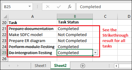
We will make a list of some tasks in a column and its corresponding column, we will create a dropdown list of the task status. This dropdown list will contain two options: Completed and Not Completed. If the task is set to Completed, it is strikethrough by a line and if not, it will be the same as earlier.
Now, the point is – how will do. Thus, see the steps given below –
Steps
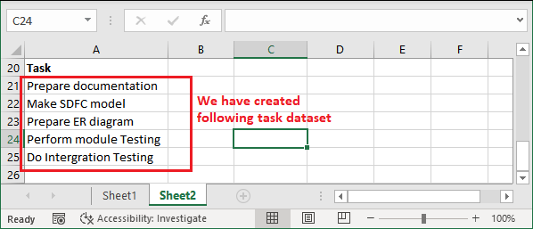
Step 1: Firstly, see the data created by us for this example.
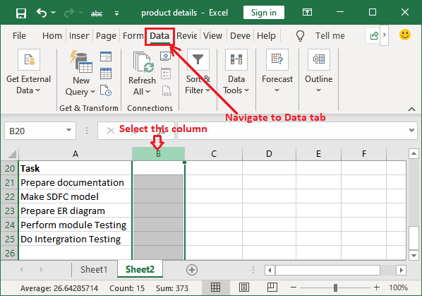
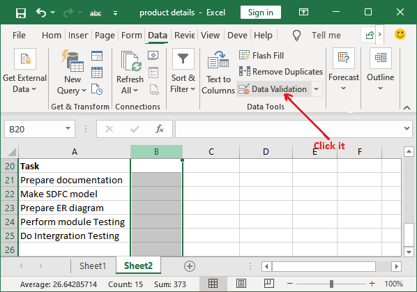
Step 2: Now, to create the dropdown list for Status column (Column B), select column B and navigate to the Data tab in the Excel ribbon.
Step 3: Click on the Data Validation that will option a validation panel to set the validations.
Step 4: Select List inside Allow dropdown field and provide Completed and Not Completed inside source field by separating them with comma.
Completed, Not Completed
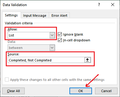
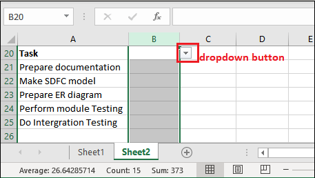
Step 5: At the end, click OK to complete this dropdown list creation process and see that a dropdown button is added on column B with value completed and not completed.
Now, we will apply conditional formatting on the dropdown button action.
Apply Conditional formatting
Step 6: Select the cells on which you apply the conditional formatting and go back to the Home tab, where you will see the Conditional Formatting option.
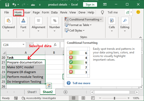
Step 7: Click on the Conditional Formatting button and then choose New Rule in the list.

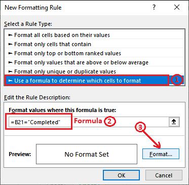
Step 8: A formatting panel will open, where choose:
- Select the Rule type: Use a formula to determine which cell to format.
- Write the formula: =B21=”Completed”
- Click the Format button now.
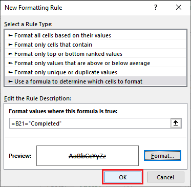
Step 9: Mark the Strikethrough option and click OK.
Step 10: When the format is set to Strikethrough, click OK here to save the conditional formatting.
Now, whenever you select Completed from the dropdown list, its corresponding task stored in column A will be strikethrough.
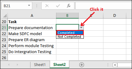
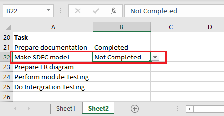
Step 11: Click on the dropdown button and select Completed for the first task stored in A21 cell.
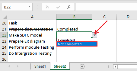
Step 12: See that the task is still visible, just a line goes through over the task that indicates that the task has been completed.

Step 13: Now, let’s choose the next task to be Not Completed and see the result.
Step 14: See that – this time task has not been strikethrough.
Step 15: Now, see the conditional formatting with strikethrough for all tasks we have created in this worksheet.