Amortization schedule template
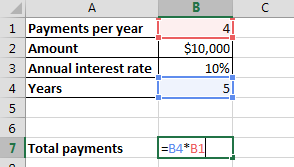 2. Make four columns (i.e. Payment number, Payment, Principal, interest and remaining balance).
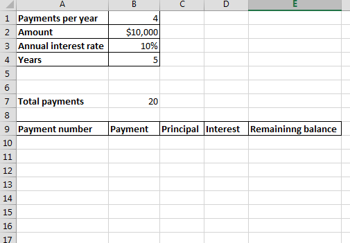
3. Write 1 in the first cell of payment number column.

4. We will use PMT function to calculate the payment.
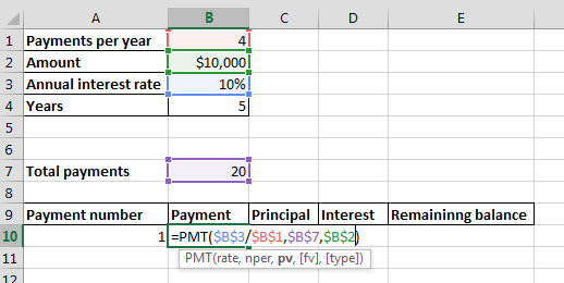
5. We will use PPMT function to calculate principal.
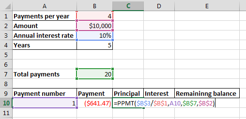
6. We will use IPMT function to calculate interest.
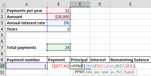
7. We will simply compare the difference between amount and payment. Since Excel by default shows payment in negative, therefore we will add the amount and payment.

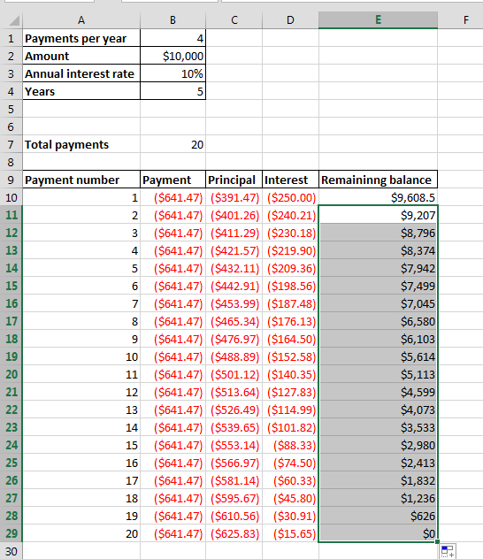
8. We will drag the first four columns (i.e. payment number, payment, principal, interest) till 20 (which is the number of Total payments). Thus, Excel will automatically calculate it.

9. Now, we will update the second row of the remaining balance column. We will add the remaining balance of the first column to the payment of the second column.

10. Finally, we will start dragging the second row of the remaining balance column to payment number 20 (which is the number of Total payments).
Template
Further reading:
Basic concepts
Getting started with Excel
Cell References


