Solver in Excel
Below is a practical example of the use of Solver to find solutions to all kinds of decision problems.
Install, Start-up the Solver Add-in and follow the process.
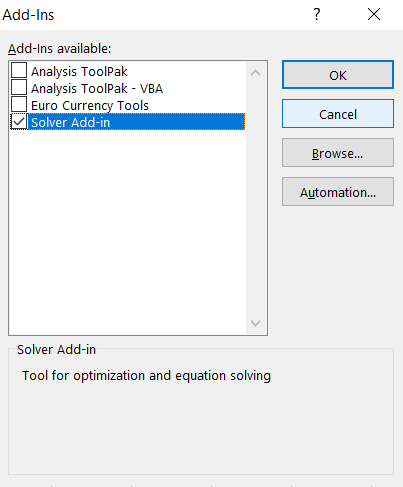
Before you begin, ensure that the Solver is already installed on your computer. Go to the menu bar and click on Data. The Solver is displayed on the right side under the Analysis. When you don’t see it, then Solver may not be installed. To install Solver tool click the Options on the green File tab. Under the Add-Ins option, click on the Solver and click on the Go button.

New dialog window appears. Choose Solver Add-in and click OK.
The Solver has been just installed and added to your Excel. Solver can be located on the Data tab under Analysis field.

After opening the Solver, a dialog box loads automatically which allows you to specify the parameters you want to run the Solver.

The parameter you specify will depend on the type of problem you want to solve. But the most common types of parameters are constraints, changing cells, and target cells.
Using Solver Tool in Excel
Okay. Now that we are through Adding Solver to the Excel features, it is time to learn how to use Solver tool in Excel. Let’s say you want to use this tool to help you solve a business problem such as running a cybercafé. The following steps will help solve this problem using Solver.
Suppose you take a bank loan to purchase UPS, furniture, and computers, and other accessories needed to successfully run a cybercafé, we can make use of the PMT function to find the amount of monthly installments needed to completely repay the bank.
The regular monthly expenses include maintenance, electricity, salaries, internet charges to the ISP, rent, advertisement costs, and telephone costs. The rented accommodation can take up to 24 computers but let’s begin with 12.

Based on the cost, the minimum amount to charge the customers can be determined. But at this point, we are not going to concern ourselves with profit. The estimates will be made for break even (because we want to repay the bank loan before looking at profits). Using the Solver and an analysis of the per hour rates obtainable in other cybercafés, a what-ifs-analysis can be done to determine what can be charged to customers.
Go to Data and select Solver. When the new window appears, select the target cell and equate its value to a certain number like 70,000 or 100,000. You may decide to set the lowest or highest value, but we won’t need to set this level in this example. If we are dealing with minimization of cost here, then the maximum and minimum option will be useful.

If you want, you can equally set the value to be zero (0), to allow you establish the break even point where the monthly earnings will be equal to the monthly expenditures.
The Final step is to determine the cells that will affect the target cell. Determine the constraints like the minimum and maximum hours of work, minimum and maximum numbers of computers. It is important to make sure that the number of computers is a whole number. You can’t have 2.4 computers because it will be difficult to analyze data. We also need to determine the lowest and highest amount that can be charged per hour for the cybercafé as determined by the research from other cybercafés. When this is done, input the necessary figures and make use of the Autosum features. You can now use the save data to manage your expenses and income until you approach breakeven for the loan collected.
Solving the Multiple Traveling Salesman Problem using Solver
Let’s calculate the Multiple Travelling Problem. This is well known mathematical problem to solve which require complicated and time consuming calculations. The Solver tool is such powerful that will find the result in less than a minute.
The clue of the Multiple Traveling Salesman Problem is to find the shortest possible path for deliveries to many places. Salesman needs to visit each city only once before going back home. Solver will calculate the proper order between cities. This is very needed in modern times when many companies struggle to use their resources the most effective way.
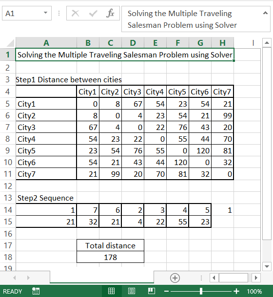
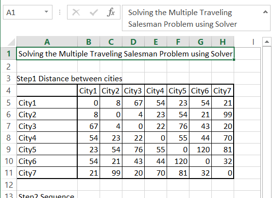
To solve the travelling salesman problem you need to prepare a matrix data. This is the distance between the cities the salesman need to visit before going back to the home city. Each city needs to be visited only once.
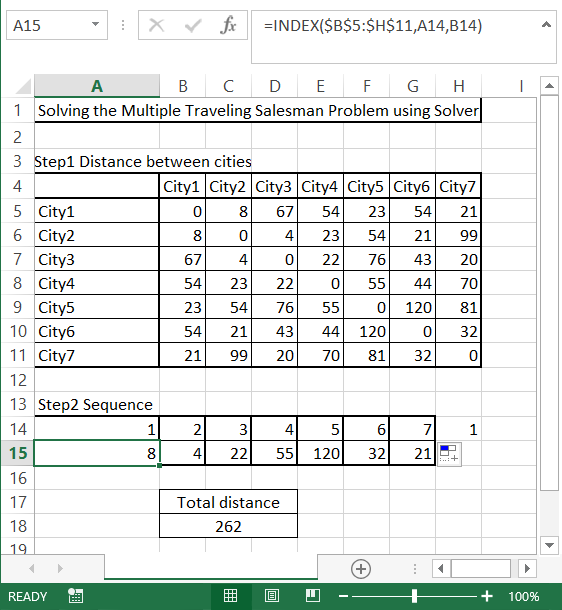
Then in next step prepare the random order of cities. In the eight column put starting city using =A14 formula. In the column below put the distance between cities using INDEX function. The formula is
=INDEX($B$5:$H$11,A14,B14)
Calculate total distance using simple SUM function. Formula here is
=SUM(A15:G15)
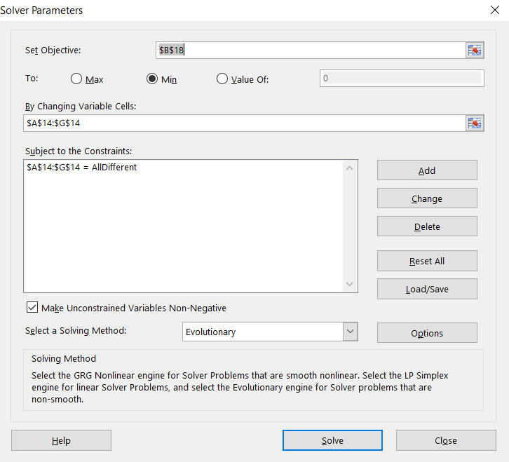
Then go to Solver and fill in like follows:
- Set Objective – minimize (Min) the Total distance ($B$18)
- By changing variable cells – Order of cities ($A$14:$G$14)
- Subject to the Constraints – add that all cities needs to be different since each city needs to be visited only once ($A$14:$G$14 = AllDifferent)
- Select a Solving Method – to get the better solution use Evolutionary
This is how to the solve the Multiple Travelling Problem to find the shortest path. Solver gives you much better solution than yours random one.