How To Put A Target Line On An Excel Chart
First we will create a simple chart showing the daily sales of a company and we will create a simple bar graph for the same.
Data creation:
This is the daily sales data for a company. As shown in Excel file:

Creating a simple bar chart from the Actual sales data:

Clicking 2D clustered column chart:
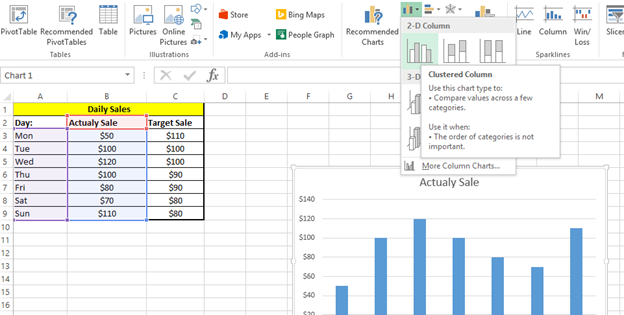
Now Adding target sales data for the target line creation. Right click the chart Area and click select Data:

Click Add for the legend entries:
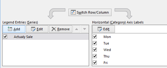
After clicking Add, select the series name by clicking cell with name target sale and select series values from column with target sales data:
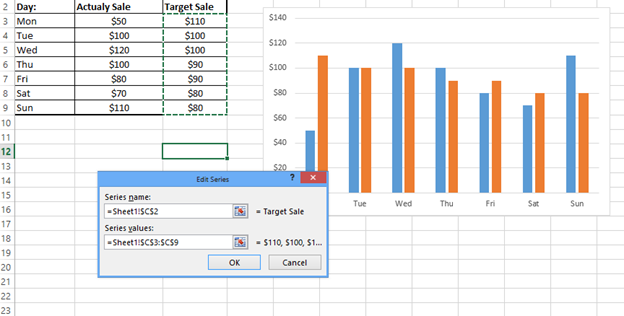
And clicking ok:
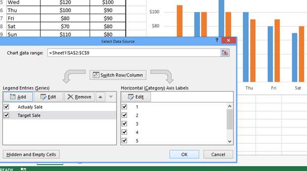
Now the target sales are added as columns but we can change the same to target line by right clicking the target series and changing chart type:

Change option for Target sale to Line:

Click Ok:
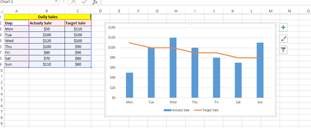
You can add legends if not shown.
Template
Further reading:
Basic concepts
Getting started with Excel
Cell References


