
Highlight Duplicates in Excel
MS Excel, abbreviated to Microsoft Excel, is extremely powerful spreadsheet software used to record financial and accounting data within different cells in multiple worksheets. It can handle a huge amount of data in each worksheet. Usually, it is a human tendency to make mistakes, and there can be cases when we may mistakenly enter duplicate values in Excel cells.
The data or values that occur more than once in the worksheet are called duplicates. Excel enables us to highlight the duplicate values to decide whether they are needed or not. We can review each duplicate and further retain or delete accordingly by highlighting these values. However, it is always recommended to keep a backup of the original Excel file before making changes to an Excel file.

This tutorial discusses the various ways to highlight duplicate values within the Excel worksheet. The tutorial explains the specific cases when we may need to highlight duplicate records.
How to highlight duplicates in Excel?
When searching for duplicate values or highlighting duplicates in Excel, the most useful and quickest way is to use the conditional formatting tool. The Conditional Formatting tool helps us to highlight duplicate values with a defined color and certain rules or conditions. The advantage of using the conditional formatting tool is that it finds and highlights existing duplicates and new duplicates to be entered in the future.
There are multiple ways of finding or highlighting duplicate values in Excel. The following are the most common and effective ways:
- Using the Conditional Formatting Rule
- Using Conditional Formatting Formula
Let us understand each method in detail:
Using the Conditional Formatting Rule
Using the conditional formatting rule, we can choose between various existing options of formatting the data within the sheet based on certain predefined rules. The tool also offers access to highlighting duplicates.
The steps to find and highlight duplicate values in Excel are listed below:
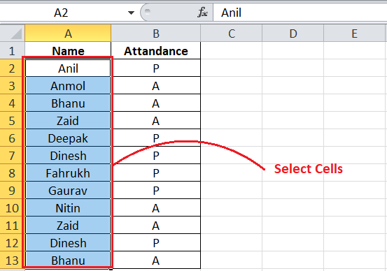
- First, we need to select the range of cells in the sheet. We can click and drag the area using the mouse to select accordingly. However, we must use the shortcut ‘Ctrl + A’ when selecting the entire worksheet.
- After selecting the data range, we must navigate the Home tab and choose the Conditional Formatting option under the Styles section, as shown below:

- In the next window (drop-down list of conditional formatting), we must click the ‘Highlight Cells Rules’ option. This option will further list more rules, where we must choose the ‘Duplicate Values’ option.
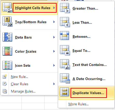
- After that, Excel will display us a dialogue box of Duplicate Values. Here, we must choose the desired color formatting option from the second drop-down, given after the ‘values with’ text. In our case, we choose the ‘Red Text’ option.

If we don’t like the predefined formatting rules, we can click the ‘Custom Format’ option from the second drop-down. This will launch the Format Cells dialogue box where we can adjust the color for text cell background, add/ remove the border, adjust border color, etc. - Lastly, we must click the OK button from the Duplicate Values dialogue box, and the duplicate values will be highlighted instantly with the red color in texts.
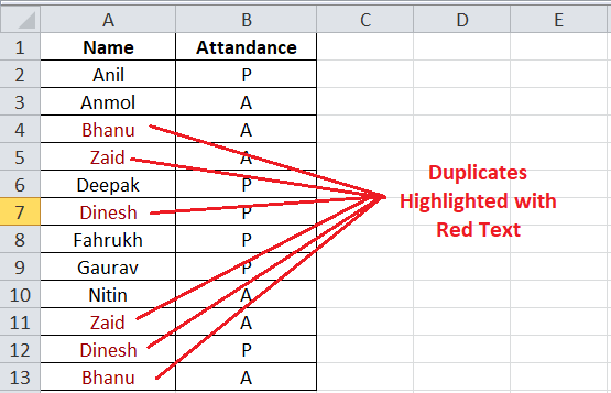
This method is mostly used to highlight repeating individual values within the selected range or entire worksheet.
Using Conditional Formatting Formula
Excel’s conditional formatting tool allows users to apply the desired formulas or functions. Using specific formulas or functions, users can target any particular range of cells and apply the desired formatting preferences accordingly. The formulas and functions help us highlight duplicates for various specific cases easily.
When highlighting duplicates in Excel using the formulas or functions, we typically use the COUNTIF function. This function returns TRUE when any specified value occurs within the supplied range more than once. For highlighting the duplicates, we apply the COUNTIF function in the following way:
The steps to find and highlight duplicate values in Excel using the conational formatting formula are listed below:
- Let’s again consider the same example. First, we need to select the effective Excel cells or a range in the worksheet. In our example, we select the range A2:A13.
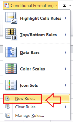
- After selecting the range, we need to go to the Home tab and click on the Conditional Formatting option as in the previous method.
- In the next window (or drop-down), we must select the ‘New Rule’ option, as shown in the following image:
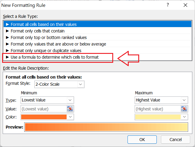
- Excel displays various options to set up a custom formatting rule for the selected cell range in the next window. Under the ‘Select a Rule Type’ box, we need to choose the last option, ‘ Use a formula to determine which cells to format’.
- As soon as we complete the previous step, Excel displays a formula window where we can type the desired formula with specific rules. We must use the COUTIF formula as below:
=COUNTIF($A$2:$A$13,A2)>1
Where ‘$A$2:$A$13’ represents the absolute reference of the selected range in our example.

- After that, we must click the Format button to launch the Format Cells dialogue box, where we can choose between various formatting options like the font color, background color, border, etc. Once all the preferences are made in the Format Cells dialogue box, we must click the OK button to close the dialogue box.

- Lastly, we must check the preview box for the selected formatting preferences in the New Formatting Rule window and click the OK button.

This will immediately highlight the duplicates within the selected range with the specified formatting. In our example, the duplicates look like this:
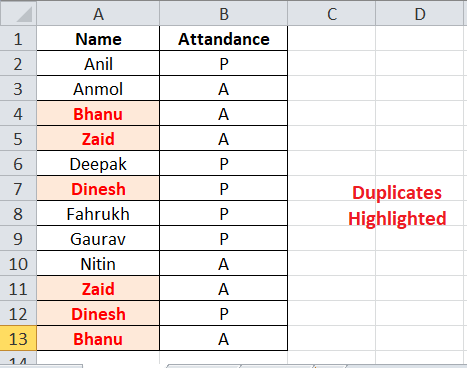
This way, we can easily highlight the repeating individual values or duplicates within the selected range or entire worksheet using the Excel formula via the conditional formatting tool. This method can also help us highlight duplicates with specific rules, such as highlighting duplicates without 1st occurrences, highlighting duplicates for 3rd, 4th, and other instances, highlighting duplicates for rows, etc.
Specific Cases for Duplicates
Using the distinct formula in the conditional formatting tool, we can highlight the duplicates based on certain use-cases. Some such common cases are discussed below:
Highlighting Duplicates without 1st Occurrences
Suppose we have multiple duplicates in our sheet, and we need to highlight the 2nd and all other subsequent duplicates in the sheet. In such a case, we must use a formula similar to this:
=COUNTIF($A$2:$A2,$A2)>1
Here, A2 refers to the top-most cell of the selected range.

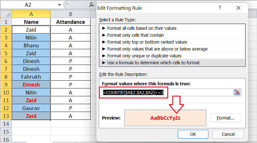
Highlighting 3rd and other Duplicate Instances
Suppose we have multiple duplicates in our sheet, and we need to highlight the 3rd and all other subsequent duplicates in the sheet. In particular, we want to highlight duplicates beginning with the Nth occurrence. In such a case, we must use the formula similar to the previous case, with only the difference that we replace >1 with the desired number. In our case, we need to apply the formula like this:
=COUNTIF($A$2:$A2,$A2)>=3
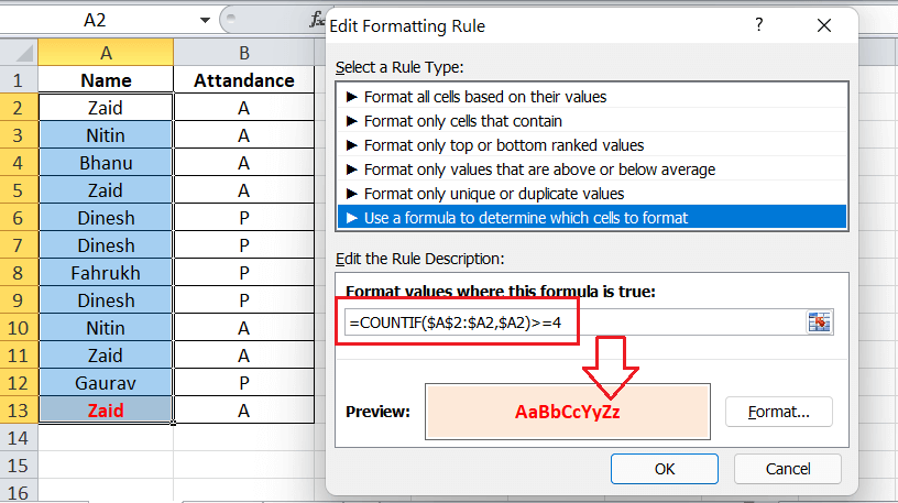
Highlighting 4th and other Duplicate Instances
Like the previous method, when highlighting 4th and all subsequent duplicates, we need to apply the formula like this:
=COUNTIF($A$2:$A2,$A2)>=4
Highlighting Specific Number of Occurrence
Suppose we have multiple duplicates in our sheet, and we only need to highlight any specific number of occurrences in the sheet. In that case, we need to use the equal sign followed by the desired number. For instance, when highlighting only the 3rd duplicate occurrence, we need to apply the formula like this:
=COUNTIF($A$2:$A2,$A2)=3
This will not highlight all the duplicate values but the 3rd of each occurrence.

Highlighting Entire Row based on Duplicates in One Column
Suppose we have an Excel sheet with multiple columns. We need to highlight the entire rows that contain duplicate values in any particular column.
Since Excel’s built-in rule of conditional formatting tool only allows us to find and highlight duplicates at only the cell level, we must use the custom formula. Using the formula-based rule, we can cover the multiple rows and columns and highlight the entire row.
To use the formula, we must select all rows and type one of the following formulas in Excel’s conditional formatting tool:
- When highlighting duplicate rows, including the 1st occurrence:
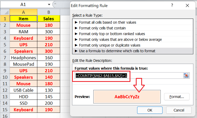
=COUNTIF($A$2:$A$15,$A2)>1
Here, A2 refers to the first cell, while A15 refers to the last cell of the specific column where we needed to check for duplicates.
- When highlighting duplicate rows excluding the 1st occurrences:
=COUNTIF($A$2:$A2,$A2)>1

The above formulas show the distinct applications of absolute and mixed cell references that made big differences for highlighting values differently.
Highlighting Equally Duplicate Rows
We highlighted the entire row based on duplicates in any specific column in the previous case. However, there may be cases where the different rows may have duplicates, meaning all the cells of particular rows may contain identical values in the sheet. We must use the COUNTIFS function instead of the COUNTIF function in such a case.
The COUNTIF function allows us to compare cells by various criteria or preferences. For instance, suppose we have an Excel sheet where two columns (A and B) have the exact values (duplicates) in some rows.
When highlighting duplicate rows in an Excel worksheet, we must use one of the following formulas in Excel’s conditional formatting tool:
- When highlighting duplicate rows with 1st occurrence:
=COUNTIFS($A$2:$A$15,$A2,$B$2:$B$15,$B2)>1
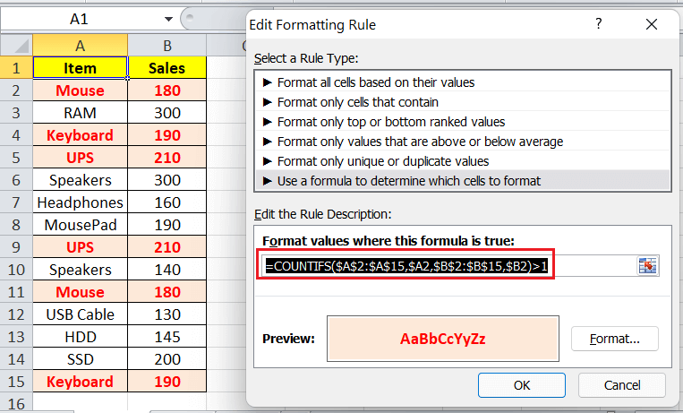
The above image demonstrates that there are duplicates for the term ‘Speakers’ in the first column, but the values in corresponding cells of specific rows are different. The function does not highlight these rows since it is only meant to highlight duplicate rows with identical values in both columns. However, the previous method helped us highlight those duplicate rows too. - When highlighting duplicate rows except 1st occurrences:
=COUNTIFS($A$2:$A2,$A2,$B$2:$B2,$B2)>1
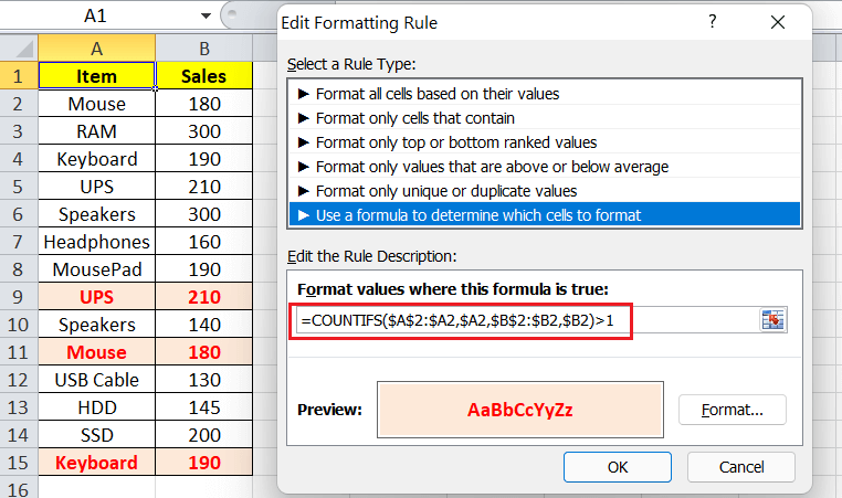
In the above example, there are only two columns. However, the sheet can have more columns with duplicate row values, and the same method will be applied. The COUNTIFS function can help us process or highlight up to a maximum of 127 range/criteria pairs.
Important Points to Remember
- Highlighting duplicates in Excel usually comes in handy when maintaining records in attendance sheets, address directories, student report cards, and other similar documents.
- We must be cautious while deleting the duplicates in the worksheet because they can impact other sheet records.
- The Format Cells dialogue box helps us to highlight the data with the desired color combinations or formatting.


