Freeze Rows in Excel

MS Excel, also known as Microsoft Excel, is popular spreadsheet software used to record large data sets in cells formed by intersecting rows and columns within worksheets. When working with large datasets within a worksheet, we can see that it becomes complicated to compare different sets of data. It becomes difficult to know what data we are reading as we scroll far beyond the header rows. In such cases, Excel’s Freeze Row option is the solution.

This tutorial discusses the essential use-cases and step-by-step methods when we may need to lock or freeze rows in Excel. This tutorial uses Excel 2010 for educational purposes; however, the methods also work on other Excel versions in the same way. Before discussing the methods, let us first understand the use of the freeze rows feature and how it helps us increase the worksheet’s effectiveness and readability.

What is the Freeze Rows feature in Excel?

Freezing Excel rows is one of the phenomenal features to increase the readability of data in a worksheet. This makes it easier to navigate the spreadsheet when we have large data sets within a sheet. When we freeze one or more desired rows in Excel, the corresponding row is locked to be visible on the screen even if we scroll the sheet to the very bottom. It is mainly helpful to compare data from different parts of the sheet.

For example, suppose we have the title or headings in the first row and the relevant data in the rows below. If we scroll the sheet, the title/headings will not be displayed, and the data will be difficult to read or understand. If we freeze the entire row with title/headings, we can easily read the data for specific headings and act accordingly.

How to freeze rows in Excel?

When freezing rows in Excel, there may be different cases. We may only need to freeze one row or the top row in most cases. But sometimes, we may need to freeze a group of rows. Excel does not limit the number of rows we can freeze, making this feature more productive when working on large data sets within a worksheet.

Let us discuss both the ways that will help us freeze rows depending on the desired use cases:

Freeze Top Row in Excel

Before moving on to the steps to freeze the top row, we must understand that this method does not typically freeze the top row of the worksheet. Instead, it freezes the first or top row that appears in the active Excel window. For example, if the visible area of our Excel window displays the 5th row at the top, the 5th row will be used as the top row or the first row. So, we should place the desired row at the top of the visible Excel window before following the below steps:

• First, we must scroll the sheet until the row we want to freeze comes at the top of the visible area. In our example sheet, we place the 5th row at the top of the visual field because we need to freeze/ lock the 5th row.
  
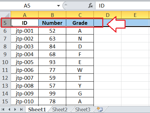
• Next, we need to navigate the View tab on the ribbon and click the drop-down arrow associated with the Freeze Panes We must select Freeze Top Row from the drop-down list, as shown below:
  
• As soon as we click on the ‘Freeze Top Row’ option, the respective row gets locked immediately. If we scroll through our sheet, we will see that the 5th row appears at the top of the Excel window while the other rows continue to scroll normally.
  
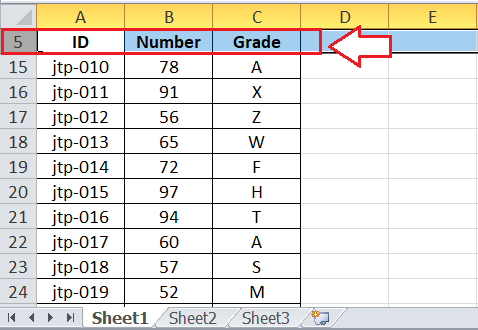
  In the image above, we can see that even after scrolling the row to the 15th row, the 5th row is fixed at the top.

Freeze Set of Rows in Excel

Excel also gives the flexibility of freezing multiple rows within the sheet, restricting the scrolling of the corresponding rows. We can easily freeze a set of rows from the top row to the desired row. However, it is essential to note that we can only freeze adjacent or contiguous rows in Excel. Excel does not allow us to freeze random rows in the middle of the spreadsheet from different parts. It means that when we are freezing multiple rows in an Excel sheet, we must also freeze/lock everything above the last frozen row simultaneously.

To freeze a set of rows, we can perform the following steps:

• First, we need to select the row right below the group of rows that we want to freeze. Suppose, if we want to freeze the first and second row in an Excel sheet, we must select the third row or a cell in the first column of the third row. We can click on the corresponding row’s header to select the entire row.
  
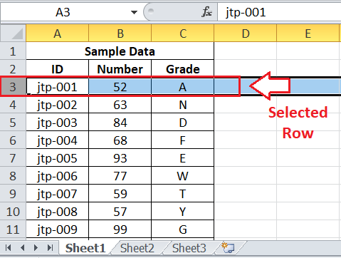
• After selecting the row, we must go to the View tab on the Excel ribbon and click the drop-down arrow associated with the Freeze Panes option. We must select the Freeze Panes option from the drop-down list, as shown below:
  
• As soon as we click on the ‘Freeze Panes’ option, the respective rows above the selected row get locked immediately. After that, if we scroll through the sheet, we will see that the first and second rows appear at the top of the Excel window while the other rows continue to scroll normally.
  
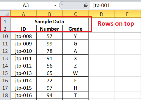
  In the image above, we can see that even after scrolling the row to the 10th row, the top two rows are fixed on the top of the Excel window.

Unfreezing an Excel Row or Multiple Rows

If we mistakenly freeze the wrong row or no longer need the rows to be frozen, we can easily unfreeze them. To unfreeze the rows from the worksheet, we can perform the following steps:

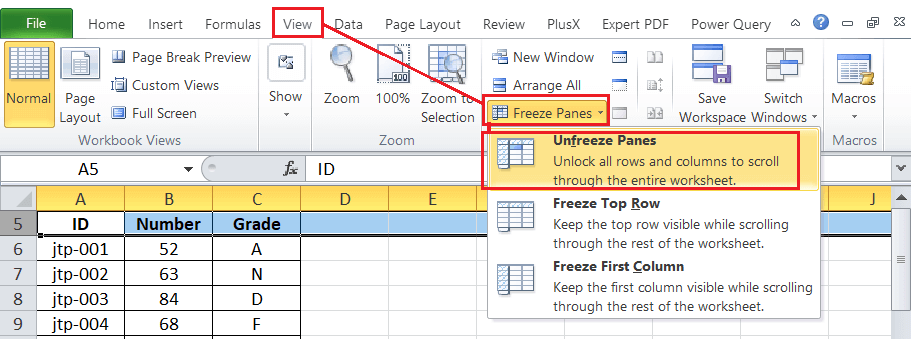
• First, we need to open the specific worksheet and navigate the View tab on the ribbon.
• Next, we must click the Free Panes drop-down arrow and select the ‘Unfreeze Panes‘ option. This will unlock all the rows and columns within the selected sheet.
  

Important Points to Remember

• When freezing a row using the View > Freeze Panes > Freeze Top Row, Excel does not technically freeze the first row of the sheet. Instead, it freezes the top row visible in the active view area of an Excel window.
• We cannot freeze non-contiguous rows in the Excel worksheet.
• While freezing a set of rows, we cannot freeze the rows anywhere from the middle of the worksheet. This means we can freeze the set of rows starting from the first row until the row’s desired number.
• It is recommended to select the entire row when freezing multiple rows. All rows above the selected row freeze. Also, if we select a cell, the Freeze tool behaves differently. If we select a cell in the first column, the rows above the selected cell are locked. If we select a cell in the first row, the columns left in the selected cell are locked. Similarly, if a cell is selected in the middle of the sheet, there are rows on the top and columns on the left; all such rows and columns will be locked.