Formula Auditing in Excel

The Formula Auditing is one of the most useful tools in Excel any entrepreneur or employee can use, especially while dealing with large volumes of data. Sometimes you are only given completed Excel worksheets on which you need to put extra analysis. Many times, it becomes difficult to notice all of the functions that are present in a file. When you land up with this situation, always use the Excel inbuilt Formula Audit toolbar.

The tutorial we will cover the definition of Formula Auditing, different methods for formula auditing and troubleshooting formulas, step-by-step analysis of each method.

What is Formula Auditing?

“Formula auditing is an essential tool in Excel that enables users to show the relationship between formulas and cells.”

Excel Formula Auditing toolbar helps the user to quickly and easily find:

• the cells contribute to calculating a formula present in the active cell.
• the formulas that refer to the active cell.

The output of Formula Auditing is presented graphically by arrow lines, thereby making the entire formula visualization effortless. It allows the user to show all the formulas in the active worksheet with a single command. In case your formulas are further referring to cells present in a different workbook, it also opens that workbook.

Microsoft Excel provides several different methods to audit a Formula. If you click on the Formulas ribbon tab of Excel, you will find the Formula Auditing section. However, many users might also need to customize the ribbon to see this option. Following are the different ways using which you can audit a formula:

1. Trace Precedents
2. Trace Dependents
3. Remove Arrows
4. Show Formulas
5. Error Checking

All these methods help you with formula auditing and troubleshooting formulas. Moving ahead in this tutorial, we will learn in detail about each method.

#1. Trace Precedents

Trace Precedents displays tracer arrows from the cells showing the direction of information flow. You see a blue box around the cells when this method is active. However, one can press this button multiple times to catch additional levels.

Let’s understand the method using an example:

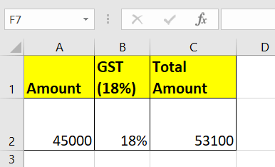
As shown in the above table, we are given formula in the D2 cell for calculating the GST amount for your Service amount.

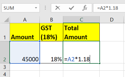
Select the required cell and press the F2 button to enable the edit mode. You will notice that the precedents cells got bordered with various colors and written in the same color and cell reference.

As a result, you will notice that cell A2 is highlighted with blue color, and the border color is also filled using the same color.

Though it is simple and easy, we have a more suitable method to check precedents for the formula cell.

Following are the steps to use Trace Precedents in your Excel worksheet:

1. Select the formula cell.
2. Go Formula option in Excel ribbon tab. In the “Formula Auditing” group click on the Trace Precedents option.
   

NOTE: If there occur no trace precedents in the cell, Excel will throw an error message.

3. As a result, you will see an arrow as shown below.
   
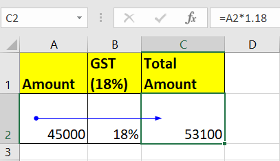
   In the above image, the precedent cells are shown with blue dots.

#2. Trace Dependents Function

This function lets the user see all the formulas in which a particular cell is used. For instance, let’s say you have a value used in multiple formulas in your Excel worksheet. In that case, you select the formula cell, click on the Trace Dependents option, and all formula cells where that same value is used will be displayed in blue with colored arrows pointing from that cell to the formulas wherever it is used.

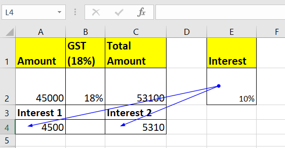
In the example below, we have calculated the 10% interest for the base amount and the GST amount.

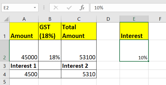
Here we have used the formula =A4*E2 for the first cell and =C4*E2 for the second cell. Therefore, we can conclude that E2 is a dependent cell for the cells A4 and C4. Following are the steps to use Trace Dependents function for the cell E2 in your Excel worksheet:

1. Select the dependent cell E2.
2. Go Formula option in Excel ribbon tab. In the “Formula Auditing” group click on the Trace Dependents option.
   
3. As a result, you will see a two-headed arrow appearing from E2 to A4 and E2 to C4, showing A4 and C4 are dependent on E2.
   
   Later, if you want to get rid of these arrows, you can use the Remove Arrows option available in the same section.

#3. Remove Arrows

In the above two options, we covered Trace Precedent and Trace Dependent. Using both methods, we have displayed tracer arrows from the cells showing the direction of information flow. But what if we want to remove the arrows afterward?

Don’t worry; Excel has provided an inbuilt option in the Formula Auditing section to remove the arrow quickly. Following are the steps to remove the arrows from the cell E2 in your Excel worksheet:

1. Go to the Formula tab in Excel ribbon tab. In the “Formula Auditing” group click on the Remove Arrow option.
   
2. As a result, all the arrows from the active Excel worksheet will disappear.
   

Note – If you want to trace dependents of a cell, make sure a formula should reference the cell in another cell; else, it will throw an error message.

#4. Showing Formulas

When you are working on an Excel worksheet that carries multiple formulas, you often need to check the formulas to ensure things are working smoothly. Excel has provided the Show Formula option in the formula auditing section to quickly display all the available formulas in your active worksheet. Sounds great, isn’t it!

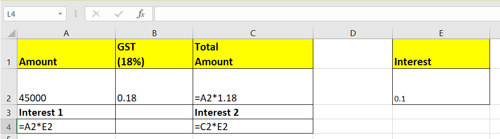
The worksheet below contains the GST report and 10% interest figure for our base amount.

Here we have entered the formula in three of the cells. Following are the steps to display all the cells containing formulas in your active Excel worksheet:

1. Go to the Formula tab in Excel ribbon tab. In the “Formula Auditing” group click on the Show Formulas option.
   
2. All the Formulas in the active worksheet will be displayed, so that at once you will get to know which cells contain formulas and what the formulas are.
   Refer to the below image to see all the formulas.
   

#5. Evaluating a Formula

Sometimes you are given a pre-made worksheet wherein complex formulas are used. To uncover the step-by-step working of a complex formula, you can utilize the Excel Evaluate Formula command.

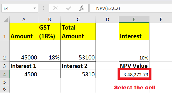
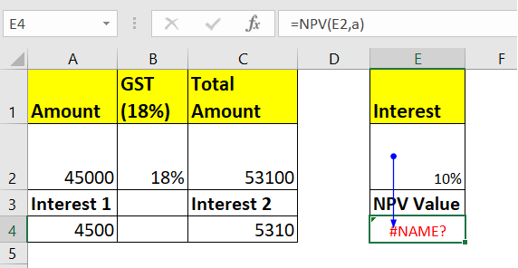
Let’s suppose we have incorporated the NPV formula in cell E4. To Evaluate the formula, follow the below-given steps:

• Click on the formula cell i.e., E4.
  
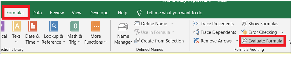
• Go to the Formula tab in Excel ribbon tab. In the “Formula Auditing” group click on the Evaluate Formula option.
  
• The Evaluate Formula dialog box will be displayed. In the Evaluate Formula dialog window, the formula used in the specified cell is displayed in the box under Evaluation.
  
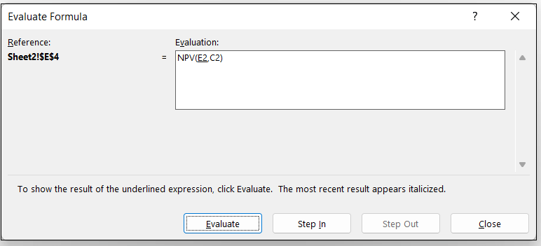
• Next, click on the Evaluate button many times. It will enable Excel to give you a step-by-step evaluation of the formula. It will show the result of the underlined expression.
  
• When you get the final output, and there will be no more expressions to evaluate, you will notice that the Evaluate button will be changed into the Restart, signifying the completion of the evaluation.

Error Checking

Errors are common when we deal with functions and formulas. Therefore, evaluating a formula is essential as it checks the specified formula or function error. It is a good practice to check all the errors in your worksheet once all the calculations are done.

Let’s understand the same using a simple calculation.

As you can see the above calculation has computed an error #NAME? in the cell E4. Following are the steps to check errors that occurs in your Excel worksheet using the Error checking method:

1. Click on the error cell i.e., E4.
   
2. Go to the Formula tab in Excel ribbon tab. In the “Formula Auditing” group click on the arrow next to Error Checking option.
   
3. In the drop-down list, you will notice three options, i.e., Error-checking, Trace errors, and Circular References. In our case, as you see, the third option is deactivated, representing that the Excel workbook contains no circular references.
   
4. Select the Trace Error option from the drop-down menu.
   
5. The cells required to compute the active cell are represented by blue arrows.
   
6. Click on Remove Arrows. Again, click on the drop-down arrow next to Error Checking option. From the drop-down list select the Error Checking option.
   
7. The Error Checking window will be displayed.
   

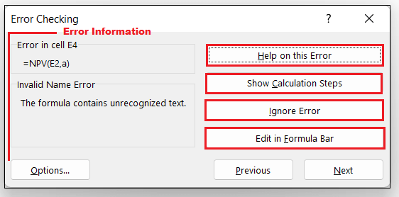
Observe the following points of the Error Checking window:?

1. All the error information will be displayed on the left side of the window pane. In our case, it has indicated that the error has occurred because our formula contains some unrecognized text.
2. The Help on this error option will direct you to the Microsoft page displaying all the steps to correct the error.
3. As the name suggests, the Show Calculation Steps option displays the Evaluate Formula dialog box.
4. If you click on the Ignore Error option, Excel will close the Error Checking window at once and if you click on Error Checking option again, Excel will ignore this error.
5. The Edit in Formula Bar option takes you to the cell formula in the formula bar, so you can further edit the formula in the cell.

Features of Formula Auditing

Below given are significant features of Formula Auditing:

• Formula Auditing allows easy Auditing of formula dependents and precedents, including object dependencies (charts, pivot tables, pivot charts, form controls, formula validation, etc)
• Formula Auditing quickly helps the user to find if them occurs any circular references in their Excel worksheet.
• It quickly helps to trace the errors.
• It lessens the time in your workbook calculation and helps to quickly to find errors in your formulas.
• Formula Auditing check columns for formula inconsistencies.
• Formula Auditing allows to check all the errors in your worksheet once all the calculations are done

Things to Remember

1. You can also show the dates in the number format if we click on the ‘Show Formulas’ option.
2. If you want to evaluate an Excel formula, you can take advantage of the shortcut key “F9”.