Excel XOR() Function
The concept of exclusive OR is more common in the world of programming. In English, we may think of a sentence like: “I’m either going to pursue Electronics Engineering or Computer Science Engineering from a reputed University”. It is clear from the sentence that the speaker cannot work on both the courses together. They can only plan to pursue only one or the other. If they pursue any one of the courses, the statement is TRUE. If they pursue neither or both, the statement is FALSE. The concept of XOR (Exclusive OR) is similar in the programming world.
This tutorial will cover the all the important aspects of Excel XOR() Function, including its syntax, parameters, return type, points to remember, examples, and many more!
What is Excel XOR Function?
“The Excel XOR function stands for “Exclusive OR”. This function returns a logical Exclusive OR of all parameters.”
If the user specifies two logical statements, the XOR function returns TRUE if either of the conditions is TRUE, but it returns a Boolean FALSE if both the conditions are TRUE. If both the statements are FALSE, it returns FALSE. If your XOR function has two or more logical values, this function returns TRUE if the count of TRUE logical is odd, else it returns Boolean FALSE.
People often confuse it with Excel OR function. But both are different. The OR function returns true if any statement is TRUE, whereas the XOR() function only returns TRUE in specific cases.
Syntax
Parameters
logical1 (required)- This parameter represents an expression or a constant value that estimates either Boolean TRUE or FALSE.
logical2 (optional)- This parameter represents an expression or a constant value that estimates either Boolean TRUE or FALSE.
Return
The Excel XOR() function returns the following outputs:
- Both the conditions are TRUE, the result is False
- IF condition is TRUE and one if FALSE, the output is TRUE
- IF condition is FALSE and other one is TRUE, the output is TRUE
- IF both the conditions are FASLE, the output is FALSE
Points to Remember
Before working on XOR function, let’s cover some important points that will help to solve the problems easily.
- The XOR Logical statements must evaluate to TRUE or FALSE, 1 or 0, in array or references that takes logical conditions.
- The Excel XOR function returns #VALUE! error if no logical values exist in the given condition.
- If the specified array or reference contains any string or blank cells, those values are ignored.
- If your XOR function has two or more logical values, this function returns TRUE if the count of TRUE logical is odd, else it returns Boolean FALSE.
- The XOR() function was introduced with version Excel 2013. Therefore if you are using an Excel version 2013, you won’t find this function.
Examples
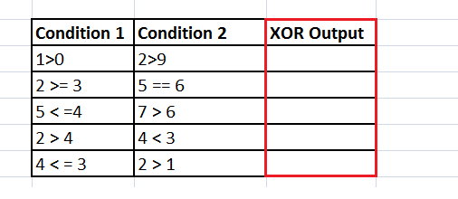
Example 1: Using Excel XOR function solve the below given conditions and fetch the outputs.
| Condition 1 | Condition 2 |
|---|---|
| 1>0 | 2>9 |
| 2 >= 3 | 5 == 6 |
| 5 < =4 | 7 > 6 |
| 2 > 4 | 4 < 3 |
| 4 < = 3 | 2 > 1 |
In the above question we are given a range of two different conditions. Follow the below-given steps to fetch the results using Excel XOR() function:
Step 1: Insert a helper column
We will add a helper column named with ‘XOR’ next to the condition 2 column.
Refer to the given below image:
In the XOR helper column we will simply use the Excel XOR() function to fetch the output.
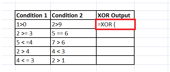
STEP 2: Type the XOR function
Move to the next column and start typing the formula. Starting with equals to(=), formula name and an open parenthesis. The formula will become = XOR (
STEP 3: Insert both the parameter
- At first it will ask to specify the first condition. Refer to the first parameter i.e, condition1 for which you want to find the exclusive OR output. So we will refer to the B4 cell. The formula will become: = XOR (B4

- Next, we will specify the second condition. So we will refer to the D4 cell. Close the bracket to finish the function.
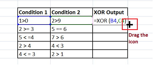
The formula will be as follows: = XOR (B4, C4)

STEP 4: Drag to copy the XOR formula across the cells
Select the cell for which you want to copy the formula. Move your mouse pointer to the end of the rectangular selection box. To your surprise the mouse pointer will convert into a small black cross icon. Drag this icon down below the cells to copy and auto-fill the formula.
Refer to the given below image:
Step 5: Excel will throw the Result
You will have the Boolean output for the given set of data. The results are fetched on the following basis:
- 1>0: TRUE, 2>9:FALSE ; Since the first condition is True and the second condition is False, the returned output will be TRUE
- 2>=3: FALSE, 5==6: FALSE ; Both the conditions are False, therefore the returned output is also False
- 5<=4: FALSE, 7>6: TRUE; Here, condition1 is False whereas condition2 is True, therefore the output will be True.
- 2>4: FALSE, 4<3 FASLE; Both the conditions are False, therefore the returned output is also False
- 4<=3: FALSE, 2>1:TRUE; the first condition is True and the second condition is False, the returned output will be False
Refer to the below image to view the result.

Example 2: Using the Excel XOR function with more than two values.
Below given is the table where we will be working with 4 different values and using the XOR function we will specify five values in a single argument instead of five separate arguments.
| C1 | C2 | C3 | C4 |
|---|---|---|---|
| 0 | 0 | 1 | 0 |
| 0 | 0 | 1 | 1 |
| 1 | 0 | 0 | 0 |
| 1 | 0 | 0 | 1 |
| 0 | 1 | 0 | 0 |
| 0 | 1 | 0 | 1 |
The XOR function is also commonly used mostly with two values. With 3 or more values, the XOR function behaves a bit different. If the users supply more than 2 conditions in this function’s argument, it will return TRUE as an output only when the number of TRUE values is odd.
Follow the below-given steps to find whether the above logical values lie in between the predictable tolerance value or not:
Step 1: Insert a helper column
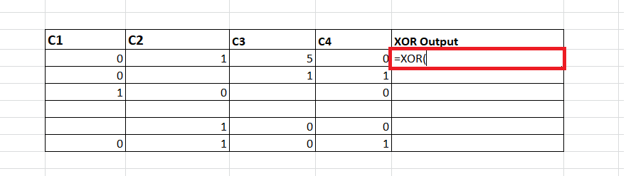
We will add a helper column named with ‘XOR output’ next to the condition 2 column.
Refer to the given below image:

In the XOR helper column we will simply use the Excel XOR() function to fetch the output for 4 different conditions.
STEP 2: Type the XOR function
In the next row, start your function with the equal to (=) sign followed by the XOR function. The formula will be as follows: = XOR (
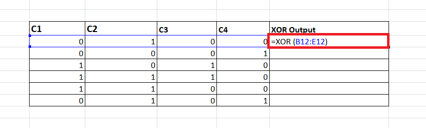
STEP 3: Insert both the range
In the parameter, we will pass the entire range like of four values in the one single argument instead of specifying five different arguments. The formula will be as follows:
=XOR (B12 : E12)
Refer to the below image:
STEP 4: Drag to copy the XOR formula across the cells
Select the cell for which you want to copy the formula. Move your mouse pointer to the end of the rectangular selection box. To your surprise the mouse pointer will convert into a small black cross icon. Drag this icon down below the cells to copy and auto-fill the formula.
Refer to the given below image:

Step 5: Excel will throw the Result
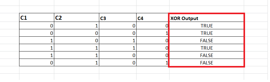
The XOR function will successfully fetch the exclusive OR for the specified numbers. The results are fetched on the following basis:
- Total TRUE cases: 1, Since the number of TRUE cases is 1, i.e., ODD, therefore the returned output will be True
- Total TRUE cases: 1, the number of TRUE logical is odd, therefore the returned output is also True
- Total TRUE cases: 2, the number of TRUE logical is even, therefore the returned output is also False
- Total TRUE cases: 3, the number of TRUE logical is odd, therefore the returned output is also True
- Total TRUE cases: 2, the number of TRUE logical is even, therefore the returned output is also False
- Total TRUE cases: 2, the number of TRUE logical is even, therefore the returned output is also False
Refer to the below image to view the resulting output for different logical conditions: