
Excel SUMPRODUCT Function
When analyzing large chunks of Excel data, you often need to count cells based on the criteria provided or find the sum after multiplying the numbers. Microsoft Excel has a special function to achieve this, the SUMPRODUCT Function, and it is a case-sensitive function that compares two strings and returns Boolean True or False.
In this tutorial, we will have a closer look at the SUMPRODUCT function and will learn the step-by-step procedure to apply this function in your Excel worksheet.
What is SUMPRODUCT Function?
The Excel SUMPRODUCT function returns the sum after multiplying numbers in an array, and it can also be used to count cells based on the criteria provided. This function is incredibly versatile and can also be used to count and sum your data, unlike the functions COUNTIFS or SUMIFS, but with more flexibility.
You can easily extend the functionality of this function by combing it with other functions with SUMPRODUCT or inserting other functions inside SUMPRODUCT. Though initially, the SUMPRODUCT function might seem harder, complex, and even pointless. But this function is an extremely versatile function with several uses. One of the reasons for using this function is that it will handle arrays smoothly, and you can utilize it to process ranges of cells in quick, elegant ways. This function is categorized under Excel Math functions.
Syntax
Parameter
Array1 (required): This parameter represents the range of cells which first need to be multiplied and then summed.
Array2 and so on..(optional): This argument represents the second array (or more arrays) or range to multiply and then summed.
Return
This function returns the sum after multiplying numbers in an array.
Points to Remember
- The SUMPRODUCT function considers all the non-numeric values in the specified arrays as zeros.
- All the specified Array parameters should be of same size else this function will throw a #VALUE! error.
- Logical tests inside arrays will create TRUE and FALSE values. In most cases, you’ll want to coerce these to 1’s and 0’s.
- You can easily incorporate other functions inside SUMPRODUCT to extend functionality of the formula.
- SUMPRODUCT can utilize the outputs of other Excel functions directly.
- SUMPRODUCT does not support wildcard characters.
Examples
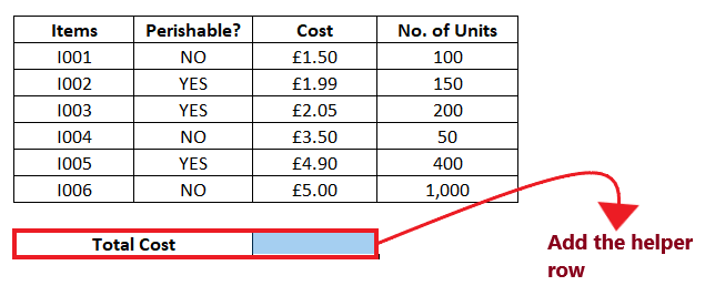
Example1: Use SUMPRODUCT function to calculate total cost faced by the superstore.
| Items | Perishable? | Cost | No. of Units |
|---|---|---|---|
| I001 | NO | £1.50 | 100 |
| I002 | YES | £1.99 | 150 |
| I003 | YES | £2.05 | 200 |
| I004 | NO | £3.50 | 50 |
| I005 | YES | £4.90 | 400 |
| I006 | NO | £5.00 | 1,000 |
Follow the below steps to use SUMPRODUCT function in your Excel worksheet:
STEP 1: Insert a helper row
Add a helper row beneath your Excel table named with “Total cost”.
It will look similar to the below image:
In the helper row, we will type the SUMPRODUCT function and calculate the cost faced by the superstore.
NOTE: As the above image shows, we have formatted the row with borders and font to make the worksheet more visually attractive.
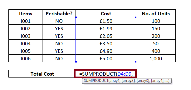
STEP 2: Insert the SUMPRODUCT formula
The next step is to enter the formula so put your cursor in the second row of your helper column start typing: = SUMPRODUCT(
It will look similar to the below image:

STEP 3: Add the parameters
- The first parameter includes “Array1,” representing the range of cells that first need to be multiplied and then summed. Here, cell range D4: D9 holds our Array1. So our formula becomes: =SUMPRODUCT (D4:D9,
It will look similar to the below image:
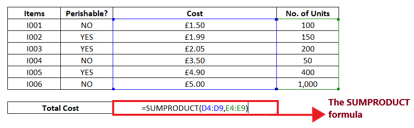
- The second parameter includes the optional arrays, but we will include only one representing the second array or range to multiply and then sum. Here, cell reference C6 holds our Text1. So our formula becomes: So our formula becomes: =SUMPRODUCT (D4:D9, E4: E9)
It will look similar to the below image:
STEP 4: SUMPRODUCT will return the result
SUMPRODUCT (D4:D9, E4: E9) will calculate the total cost faced by the superstore and return the sum value after multiplying numbers in an array.
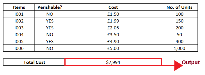
It will look similar to the below image:
Explanation of above formula
Let’s understand the mechanism (in terms of maths) with which the SUMPRODUCT works:
- The SUMPRODUCT function will take the first element from the first specified array and multiply it by the first element in the second array. Next, it takes the second element from the first array and multiplies it by the second element in the second array, and so on it continues till it reaches the last number.
- When all the array numbers are multiplied, the function adds all the products and finally returns the sum as its output.
In mathematical terms, the SUMPRODUCT formula executes the given-below operation:
Just imagine how important this function could be if your excel worksheet contains hundreds or thousands of rows!
Example 2: Use SUMPRODUCT function to count total number of Perishable items and its cost.
| Items | Perishable? | Total Cost |
|---|---|---|
| I001 | NO | £150 |
| I002 | YES | £299 |
| I003 | YES | £410 |
| I004 | NO | £175 |
| I005 | YES | £1,960 |
| I006 | NO | £5,000 |
Follow the below given steps to count the total number of perishable items (where Perishable = YES) and its cost in the above table using Excel SUMPRODUCT function:
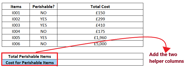
STEP 1: Insert two helper row
Add two helper rows beneath your Excel table one named with “Total Perishable items” and another named with “Cost for Perishable items”.
It will look similar to the below image:
- In the first helper row, we will use the SUMPRODUCT function to determine how many total Perishable items are present in our table.
- In the second helper row, we will type the SUMPRODUCT function and calculate the cost of perishable items.
NOTE: As the above image shows, we have formatted the row with borders and font to make the worksheet more visually attractive.
STEP 2: Insert the SUMPRODUCT formula to find count of perishable items
- The next step is to enter the formula so put your cursor in the second row of your helper column start typing: = SUMPRODUCT(
- The first parameter includes “Array1” which represents the range of cells that must be multiplied and then summed. Here, the range is referred to from cell address C5: C10. Since we have to find only the perishable items, we will equate them with “YES”.
So our formula becomes: =SUMPRODUCT(–(C5:C10=”YES”))
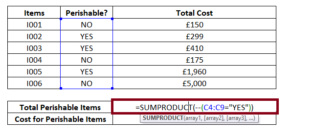
NOTE: Using two minus signs (–) in Excel, return the value of “TRUE” into 1 and “False” into 0.
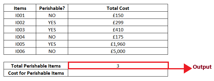
- The SUMPRODUCT function will return the count of the perishable items. Refer to the below image:
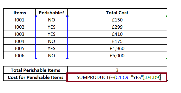
STEP 3: Insert the second SUMPRODUCT formula to find the cost of perishable items
- Enter the SUMPRODUCT formula in the second helper row: = SUMPRODUCT(
- The first parameter includes “Array1″ which represents the range of cells that must be multiplied and then summed. Here, the range is referred to from cell address C2: C10. So our formula becomes: =SUMPRODUCT(–(C4:C9=”YES”),
- The second parameter includes the optional arrays, but we will include only one representing the second array or range to multiply and then sum. Here, the range is referred to from cell address D4:D9. So our formula becomes: =SUMPRODUCT(–(C4:C9=”YES”),D4:D9)
It will look similar to the below image:
STEP 4: SUMPRODUCT will return the result
SUMPRODUCT (–(C4:C9=”YES”),D4:D9) will calculate the cost of the perishable items and return the sum value after multiplying numbers in an array. The output will be $2,669.
Refer to the below image:

Example 3: Using the SUMPRODUCT function calculate the product (soft toys) details from the below given table and find its revenue for the year.
| Products | Revenue |
|---|---|
| SOFT TOYS | 200 |
| soft toys | 400 |
| creative toys | 320 |
As shown in the above table, we have two values named with soft toys with the only difference that one is in lowercase (soft toys) and the other value in uppercase (SOFT TOYS). But we want the lowercase data value “soft toys”. However, there are other Excel functions such as VLOOKUP and INDEX/MATCH to look for the given values, but the only problem is that it is not case-sensitive. So, we will use a combination of “SUMPRODUCT + EXACT” to achieve a case-sensitive lookup.
Follow the below-given steps to product details and revenue for soft toys:
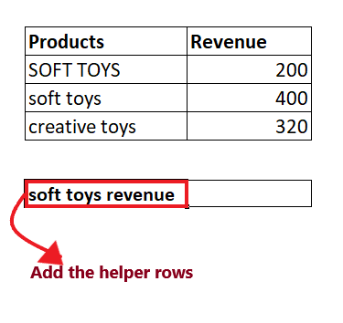
STEP 1: Insert a helper row named “soft toys revenue”
Place your cursor anywhere under products table and type the row name “soft toys revenue” on top of the cell.
It will look similar to the below image:
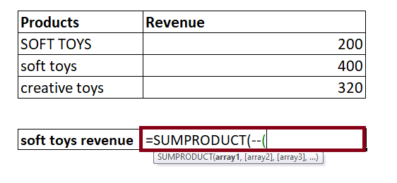
In the helper column, we will type the combination of the SUMPRODUCT + EXACT function to find the revenue details.
STEP 2: Insert the SUMPRODUCT formula
- The next step is to enter the formula so put your cursor in the second row of your helper column start typing: = SUMPRODUCT(
It will look similar to the below image:

NOTE: Excel SUMPRODUCT function returns the sum after multiplying numbers in an array, and it can also be used to count cells based on the criteria provided. This function takes arrays as its parameters.
- Before inserting the parameters, add two negative signs. We have used a double negative to convert the output TRUE & FALSE values to 1’s and 0’s. So our formula becomes: =SUMPRODUCT(–(
Refer to the below image:
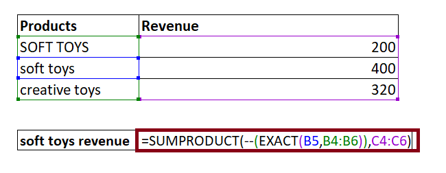
STEP 3: Insert the EXACT function as the first parameter of SUMPRODUCT
- In the first parameter, we will type the EXACT function. So our formula becomes: =SUMPRODUCT(–(EXACT(
- Next, we will pass the parameters of EXACT. In the first parameter, we will pass the string which you want to check. Here, cell reference B4 holds our Text1. So our formula becomes: =SUMPRODUCT(–(EXACT(B5,
- In the next parameter, we will pass the products name from which you want to test against. So our formula becomes: =SUMPRODUCT(–(EXACT(B5, B4:B6)
It will look similar to the below image:

STEP 4: Insert the second parameter of SUMPRODUCT
Enter the revenue range as the second parameter of SUMPRODUCT. Here, cell range C4:C6 holds the revenue range. So our formula becomes: =SUMPRODUCT(–(EXACT(B5,B4:B6)),C4:C6).
It will look similar to the below image:
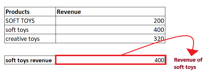
STEP 5: Combination of Excel SUMPRODUCT and EXCAT function will return the result
EXACT will return the output for the formula after running a test on the values in column B, convert the TRUE/FALSE (output of the EXACT function) to 1’s and 0’s. As shown below, using the combination of SUMPRODUCT and EXACT, you will have the revenue for ‘soft toys’ product.
It will look similar to the below image:
Eureka! Now you have successfully covered all the steps and examples for the SUMPRODUCT function. Go ahead, use it whenever you need to do any comparison, combine it with other functions and fetch satisfactory results.


