
Excel Slicer
What is an Excel slicer?
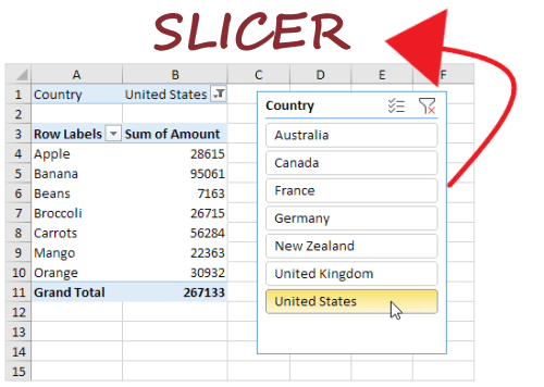
Excel Slicers are powerful for applying filters for Excel tables, pivot tables, and pivot charts. They are widely used to create attractive dashboards and summary reports because it is effortless to create, is visually pleasing and the users can use them anytime anywhere to filter their data faster and easier.
Slicer’s feature was not available in the early versions of Excel. They were initially introduced in Excel 2010 and became available in Excel 2013 and all the later versions.
Difference between Excel slicers and PivotTable filters
Slicers and pivot table filters perform identical operations, i.e., display some data and hide others. The difference between Excel Slicers and Pivot Table filters is as follows:
| S.NO. | Excel Slicers | Pivot Table Filters |
|---|---|---|
| 1. | Excel slicers have made the filtering process very easy. In the pivot table applying a slicer filter is as effortless as clicking a button. | Pivot table filters are a bit complicated when compared to slicers. Filter fields don’t specify any simple method to tell what is being filtered when the user selects two or more elements. |
| 2. | Slicers can be tied to multiple pivot tables present in the same Excel worksheet. | Filters can be connected to one pivot table only. |
| 3. | Slicers are also termed floating objects as they can be moved anywhere in the Excel sheet, such as you can keep the slicer next to your pivot table, pivot chart or within the chart area. | Pivot Filters have limited access and can only be applied to columns and rows. |
| 4. | Slicers are user-friendly and provide an interface that can perform impeccably in various touch screen environments. Though it is not fully supported for Excel mobiles such as Android and iOS. | Pivot table filters don’t work correctly on touch screens. |
| 5. | Slicers take up more Excel space. | Pivot table report filters are compact |
| 6. | Automating Slicers is tough and requires technical skills and efforts. | Automating Pivot table filters is simple and can be done easily through VBA |
Insert slicer in Excel
Slicers can be easily inserted into your Excel Tables, Pivot Tables, and Pivot Charts. Follow the below step-by-step implementation to add Slicer to your Excel worksheet.
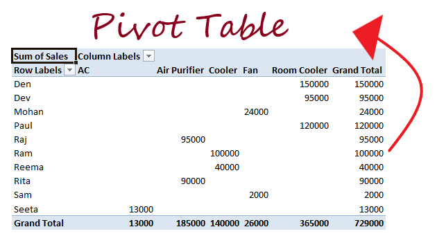
Add slicer to your pivot table
For implementing slicer in your Excel, firstly you need to create a pivot table and follow the below given steps:
- Click on your Excel pivot table.
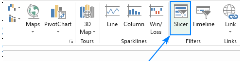
- Go to Analyze tab-> Filter group, and click the Insert Slicer option.

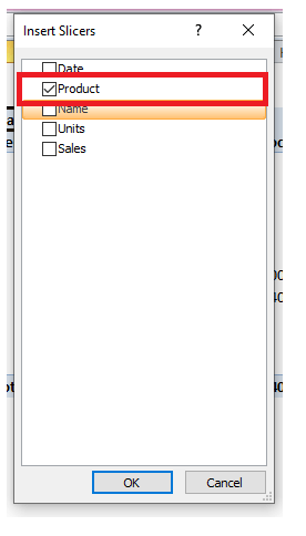
- The Insert Slicers window will be immediately displayed. It will show various checkboxes where each represents a field of your pivot table. You can select one or multiple fields for which you wish to apply the slicer.

- Click OK.
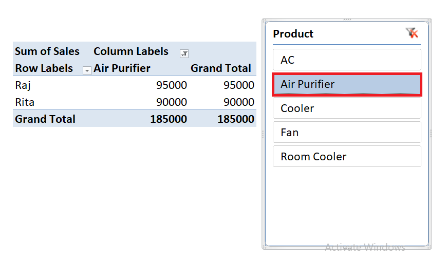
Result:
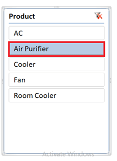
As an example, we have added only one slicer to filter our pivot table, i.e., by Product:
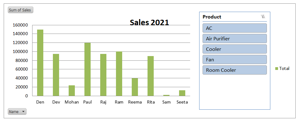
We can filter the product fields and can visualize the data of any particular. For instance, in the below screenshot, we have fetched the data for the Air Purifier Product using Slicer.
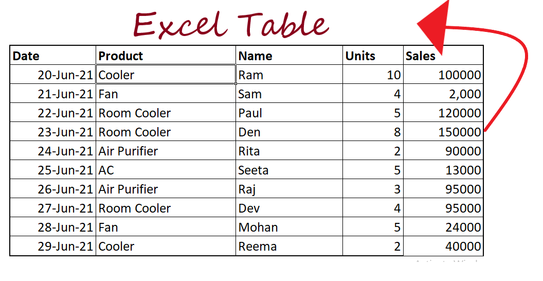
Add slicer to your Excel table
In the earlier section, we discovered how to create a slicer for pivot tables but do you know the latest versions of Excel allows the user to insert a slicer for an Excel table as well. Follow the below steps:
- Create an Excel Table and click on it.
- On the Insert tab, in the Filter group, click the Insert Slicer.
- The Insert Slicers window box will be displayed, tick off the check boxes the columns that you wish to filter. Click OK.
Add a slicer for pivot chart
In addition to the pivot table and Excel table, you can also insert Sliver to your Pivot chart and can apply a filter to them. Though you can also create a slicer for your pivot table by following the above guidelines and further can use it to filter both the pivot table and the pivot chart.
To insert a slicer with your pivot chart follow the below steps:
- Create a pivot chart and click anywhere on it.
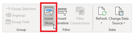
- Click on the Analyze tab. Under the Filter group, choose the Insert Slicer option.
- The Insert Slicers window will be immediately displayed. It will show various checkboxes where each represents a field of your pivot table. You can select one or multiple fields for which you wish to apply the slicer.
- Click on OK
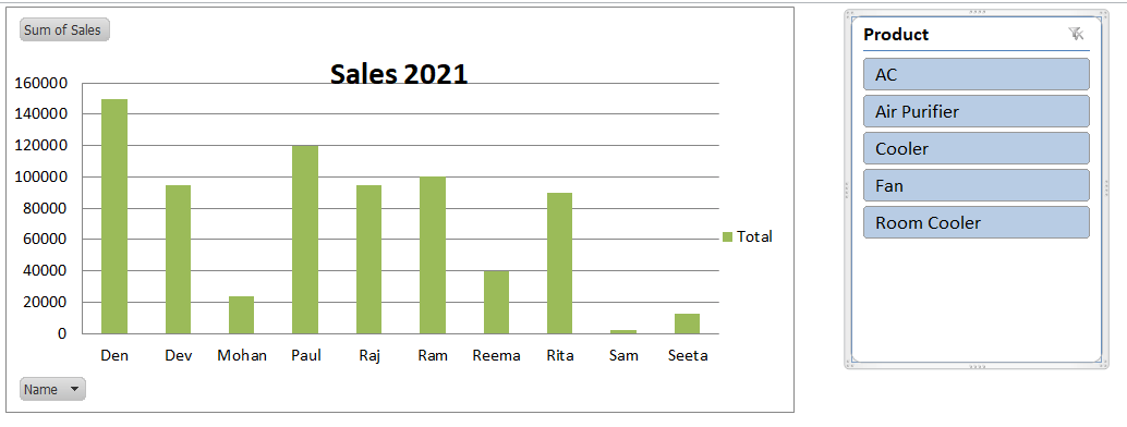
Result:
This will integrate the slicer window in your worksheet:
Please note that you can customize the appearance of the slicer box in your pivot chart. For example: you can locate the slicer window within your pivot chart area as shown below.
To incorporate the Slicer box inside the chart area, we need to increase the overall chart area and need to decrease the plot area by dragging the borders, and finally drag and drop the slicer window to the empty space:
How to Move a slicer in
You can easily move and position your Slicer to place in Excel within the same worksheet. Place your cursor on the top of the slicer unless the cursor changes to a four-headed arrow.
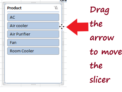
Using the arrow drag the slicer to your preferred position.
Resize a slicer
Unlike Excel Tables, pivot tables, and pivot charts, you can resize the size of Slicer as well. The most common way to change the size of the Slicer is by dragging the edges of the Slicer.
The second way is by changing the Position and Layout setting and setting it to the required height and width for your Slicer. Right-click on the top of your Slicer. The window will appear. Select the Size and Properties option.
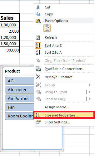
Again the Size and Properties window will be displayed. From the side pane, choose the ‘Position and Layout’ option. Set the various fields as per your requirement.
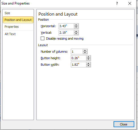
That’s it! The slicer will be set to the specified position in your Excel worksheet.
Lock the slicer position in Excel
Sometimes we need to fix the place of a slicer in your Excel worksheet. To fix the Slicer, you need to lock it in Excel. Follow the below steps:
- Create your Excel Slicer and right-click on the top of it. The following window will appear. Choose the Size and Properties option.
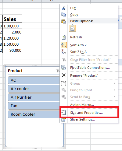
- The Size and Properties windowpane will be displayed. On the side pane, select the Properties option.
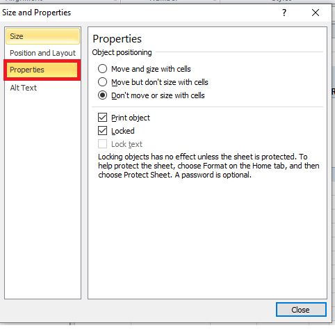
- It will display the object positioning option; select the third radio option, ‘Don’t move or size with cells box’. Close the window pane.
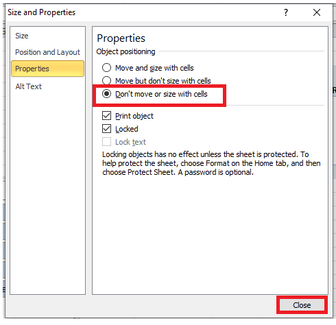
After doing this, the position of your Slicer will be locked. Even if you add or delete a new row or column or add more fields to your pivot table, the position of your Slicer will remain intact.
How to remove a slicer from a worksheet
There are two ways to delete a slicer permanently from your Excel worksheet.
Method 1
- Click on the top of your slicer to select it, and from your keyboard, press the Delete key.
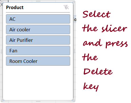
- Your slicer will be successfully deleted from your Excel worksheet.
Method 2
- Right-click on the top of your slicer. The following dialog box will appear. Choose the Remove ‘Slicer Name’ option.
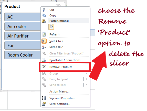
- Your slicer will be successfully deleted from your Excel worksheet.


