Excel Relative Referencing

Microsoft Excel, abbreviated as Excel, is a widely used spreadsheet software that helps users record vast amounts of data types in cells across multiple worksheets in a workbook. It enables the users to perform various simple to complex calculations on the recorded data within the cells and get the results concluded using the inbuilt functions or formulas.

In particular, most Excel formulas can be used with the desired values as direct arguments. However, we often supply corresponding cell references in Excel formulas that hold effective values needed to be used in calculations or financial analysis. The main advantage of using cell references instead of direct values in a formula is that we get real-time results or outputs by applied formulas when we change the values in the corresponding cells accordingly. There are mainly three types of cell references in Excel: relative, absolute, and mixed references.

In this tutorial, we discuss a brief introduction to Excel Relative Referencing. The tutorial also discusses step-by-step procedures for creating or using relative references within the Excel worksheets with the help of relevant examples. Before we look at Relative References in Excel, let us first understand Cell Reference in Excel with its definition.

What is a Cell Reference?

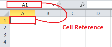
In Excel, a cell reference is defined as the name or address of a specific cell or range. It accordingly remains unique for each respective Excel cell. An Excel cell reference is formed by combining a particular column name and the corresponding row number. For example, A1 is the cell reference to the first cell in the sheet where the letter ‘A’ represents the first column and the numeric ‘1’ represents the first row of the sheet.

The primary purpose of a cell reference in Excel is to tell an Excel formula where to look for the desired value/data to be used in the formula to produce the corresponding output. In Excel, we can use cell references to refer to the same sheet, another sheet, another workbook, and many other similar programs.

What is the Relative Reference in Excel?

Relative reference is the default approach used by Excel. It makes the Excel cells reference-free, giving the fill function freedom to continue its order without any restriction. In particular, a relative reference in Excel refers to a pointer to any specific cell or range of multiple cells within the same sheet, another sheet, or workbook. For example, the relative reference for the cell A1 can be given as below:

=A1

As shown above, the relative reference in Excel is nothing but only the combination of a respective column name and row number. If we copy-paste the relative references in different cells, their references automatically change depending on the relative position of rows and columns. Relative references typically change when copied to other locations because they describe the “offset” to other cells accordingly, rather than fixed addresses.

For example, if you copy the formula (=A1*B1) from the first row to the second row of the sheet, the formula will become (=A2*B2). The relative references are mainly useful if there is a need for using the same formula or calculation in multiple cells within the workbook (s).

When do the relative references in Excel change?

As discussed above, the relative references are the default reference type used by Excel. When we use relative references, they automatically change after copying them to another location in the sheet or workbook. Each referred cell with relative reference changes with left, right, top or bottom movement.

For example, suppose we give relative reference to cell D9 and perform the movement in the following ways within the sheet:

• Leftward: The given reference (D9) automatically changes to C9.
• Rightward: The given reference (D9) automatically changes to E9.
• Upward (Top): The given reference (D9) automatically changes to D8.
• Downward (Bottom): The given reference (D9) automatically changes to D10.

How to create/ make relative references in Excel?

To create or make a relative reference, we should include the equal sign before the cell reference to refer to any specific cell in the sheet. Depending on the requirement for our formula, we can either refer to a cell or a range. Below are the steps explaining how to create a basic relative reference in Excel:

• First, we need to select a cell where we want to use relative reference for any specific cell. For example purpose, we select the cell D3 in our example sheet, as shown below:
  
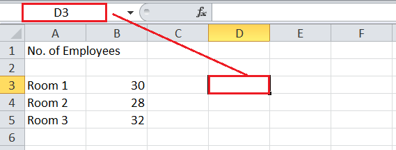
• In the next step, we must start entering the equal sign (=) and then select or type the desired point of reference (cell or range). We type the equal sign “=” in cell D3 and select cell B3 as a reference point in our example.
  
• After pressing the Enter key, we see that the same value is displayed in cell D3 as cell B3. Moreover, if we change the value in cell B3, the value in cell D3 will change accordingly. That’s because we have created a relative reference of cell B3 in cell D3.
  

How to use relative references in Excel?

Let us now understand the concept of Excel relative referencing better with the help of the below examples:

Relative Referencing in Excel: Example 1

Consider the following sheet as an example data set where numbers in four different cells, A1, A2, B1, and B2, are recorded.

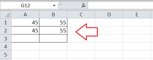
Suppose we need to SUM values in A1 and A2 in the below cell A3. Likewise, we also need to SUM values in B1 and B2 in cell B3.

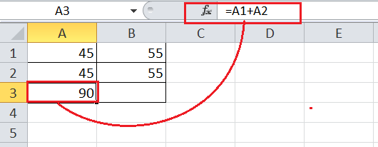
• First, we calculate the sum of two numbers from A1 and A2 in cell A3. We select cell A3, type the enter sign (=), and then select cell A1. After that, we enter the addition operator, select cell A2, and press the Enter key on the keyboard. So, the formula (=A1+A2) gives the output SUM as 90.
  
• Next, we calculate the sum of two numbers or numerics from B1 and B2 in cell B3. Since we have a similar scenario in the next column B, we can again use the addition operator to SUM values and obtain results.
  However, we can get the result in another way which will be comparatively easier and more useful when there are more similar scenarios in the next columns.
• Instead of entering the entire formula again, we can usually copy-paste (or drag using the Fill Handle) the formula from cell A3 into cell B3. When we copy-paste the contents from cell A3 to cell B3, only the applied formula is copied from one cell to another (not the result).
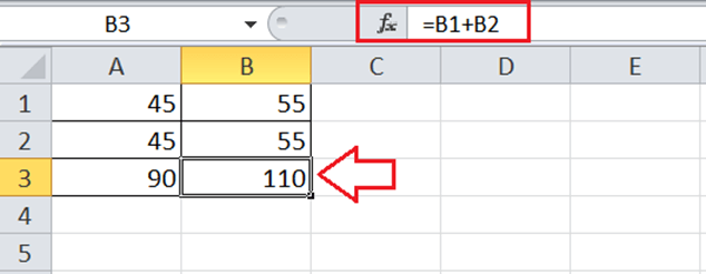
  The above image shows that the formula has automatically adopted the respective cells accordingly. After being copied, the applied formula (=A1+A2) has automatically changed into formula (=B1+B2). The cell references automatically changed based on the relative position of the row and column. However, we get the appropriate results. That’s because the destination cell B3 only contains the formula, not the source value. This is how Excel’s relative referencing works.

Relative Referencing in Excel: Example 2

Consider the following Excel sheet as an example data set where we list different items with their prices and sold quantities.

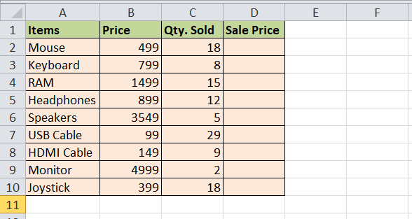
We need to calculate the Sale Price/Value for each item separately in column D. To do this, we need to multiply the sold quantities by their respective price.

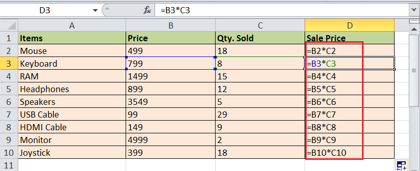
• First, we calculate the Sale Price for the first item (i.e., Mouse). So, we select the corresponding resultant cell D2 and insert the multiplication formula. We first type equal sign (=), then we select a cell with Price (B2), insert the multiplication operator (*), select the cell with quantity sold (C2), and press the Enter key. This gives the Sale Price for the first item.
  
• Next, we need to calculate the Sale Price for other items. We can apply the multiplication formula to other resultant cells similarly. However, it will take a lot of time. Therefore, we leverage the Relative Reference feature of Excel and usually copy-paste (or drag using Fill Handle) the formula from D2 to other remaining cells. This immediately calculates the Sale Price for other items in the column.
  
  Suppose we check the formula in any other specific resultant cell in column D. We notice that the cell references have changed relatively (based on relative positions of row and column) while keeping the same formula as the source cell.
  

Important Points to Remember

• The relative reference does not contain a dollar ($) sign.
• Neither a row nor a column is fixed in Excel relative referencing. If a row or column is fixed, the reference will be referred to as a mixed reference. If both row and column are fixed, it becomes an absolute reference.
• We can change between different cell references by pressing the ‘F4’ function key after placing the cursor between the specific cell in the formula bar.