
Excel IFS Function
While working with Excel worksheets, you often need multiple IFs in your worksheet. Instead of repeating the IF function, Microsoft Excel provides the inbuilt function known IFS function. The Excel IFS function is a logical function used to apply multiple IF functions. This function permits the users to test multiple conditions.
This tutorial will cover detailed information about IFS functions, their syntax, parameters, and return values. We will solve examples using the IFS function to look at the overview of how this function is used in Excel.
What is IFS Function?
“The Excel IFS function can run multiple tests and return a value corresponding to the first TRUE result. Excel users incorporate the IFS function in their worksheets to evaluate multiple conditions without multiple nested IF statements.“
The IFS function estimates multiple conditions and returns an output corresponding to the first TRUE value. You can utilize the IFS function when you want a self-contained formula to test various conditions simultaneously without nesting multiple IF statements. The advantage of using the IFS function is it creates a short formula that is easy to read and write.
Though you can provide multiple conditions to the IFS function as test/value pairs, the upper limit of this function is up to 127 conditions. Each test symbolizes a logical test that returns either Boolean TRUE or FALSE, and the corresponding value will be returned if any of the specified tests returns TRUE. If more than one condition returns TRUE, this function returns the first value corresponding to the first TRUE result. For this reason, it is essential to evaluate the order in which conditions are arranged in the formula.
Syntax
=IFS (test1, value1, [test2, value2], …)
Parameter
- test1 (required)– This parameter represents the first logical test.
- value1 (required)– This parameter represents the output when test1 is TRUE.
- test2 (optional)– Unlike the test1 parameter, it represents the second logical test.
- value2 (optional): This parameter represents the value pair for test2
Return
The Excel IFS function returns a value corresponding to the first TRUE result
Examples:
#IFS Example1: Using Excel IFS function, figure out the grades for the specified students marks in the below table.
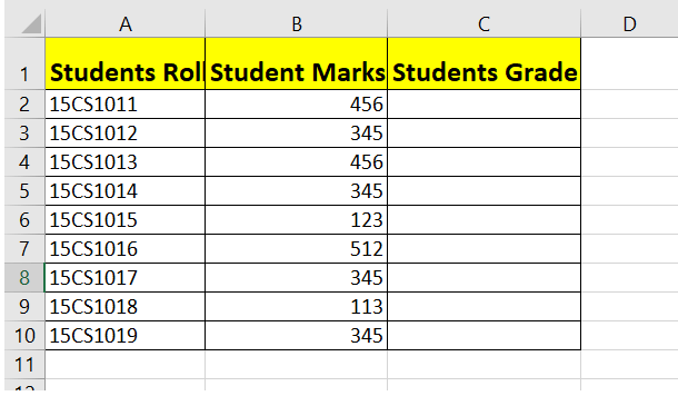
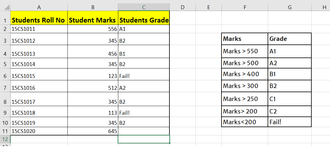
In the below table, we are given three fields, i.e., in column A, we have ‘Student Roll Number,’ in Column B, we have ‘Student Marks,’ and in Column C, we have the student’s grade. Based on the ‘Student Marks’ column, compute the grades of students who have to assign a specific remark against each student in the data set.
| Marks | Grade |
|---|---|
| Marks > 550 | A1 |
| Marks > 500 | A2 |
| Marks > 400 | B1 |
| Marks > 300 | B2 |
| Marks > 250 | C1 |
| Marks> 200 | C2 |
| Marks<200 | Fail! |
Follow the below-given steps to run multiple tests and return a value corresponding to the first TRUE result using the Excel IFS() function:
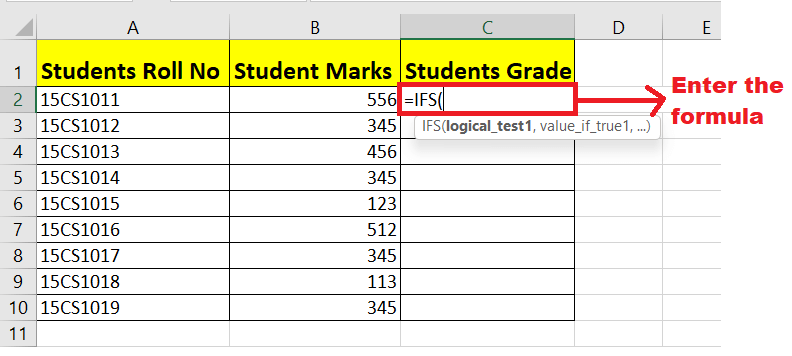
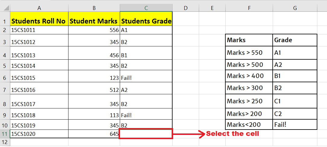
Step 1: Select a cell to calculate student’s Grade
Place your mouse cursor in the in the first cell of Score column so we can enter the formula and find the Grade for the specified marks as per the above score table. In our case, we have selected cell C2 of our Excel worksheet.
Refer to the given below image:

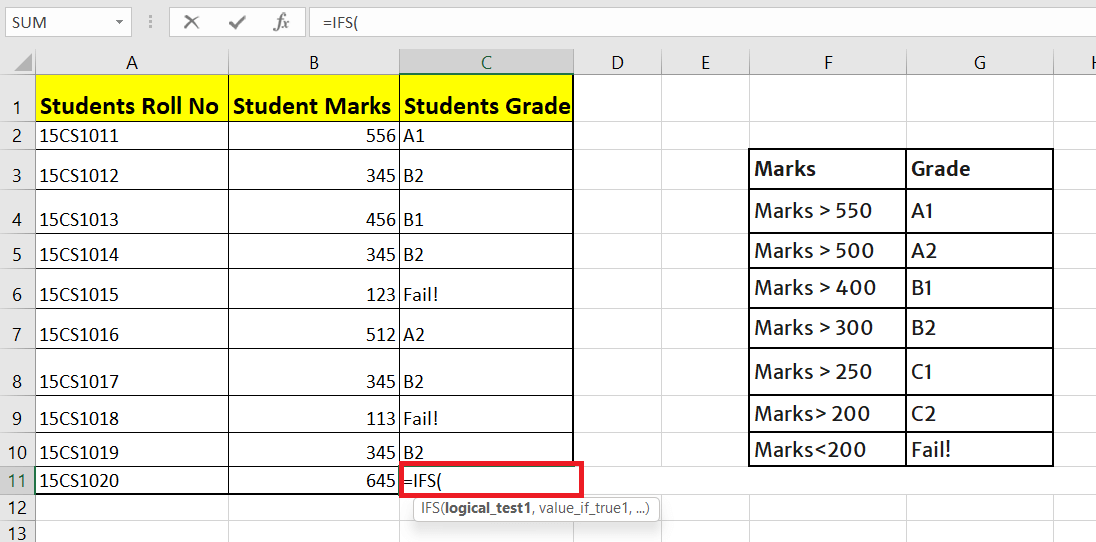
STEP 2: Enter the IFS function
To figure out the grade based on the grade chart. Start the formula using the equal to (=) sign followed by the built-in Excel IFS function.
STEP 3: Insert all the parameters
- Initially, you have to specify the first test parameter. Here, we will specify marks > 550. The formula will be =IFS(B2>550,
- Next, we will specify the value parameter that will be returned if the above test parameter evaluates TRUE. The formula will be =IFS(B2>550, “A1”,
- Similarly, we will specify the subsequent test and value parameter to satisfy the further conditions.
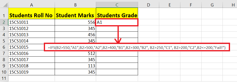
The overall formula becomes:
=IFS(B2>550,”A1″,B2>500,”A2″,B2>400,”B1″,B2>300,”B2″, B2>250,”C1″, B2>200,”C2″,B2<=200,”Fail!”)
Step 4: The IFS function will return the Grade
As a result, the IFS function will return the grade A1 since the marks are greater than 550.
Step 5: Drag the IFS formula to the following cells
Select the C2 formula cell and take the mouse pointer towards the right corner of the selected box. You will notice that towards the right side, the cursor will change into a plus (+) icon.
Drag the icon to the following cells, and to your surprise formula will be replicated to all the cells changing the reference cells accordingly. It will return the grades as per the grade table.
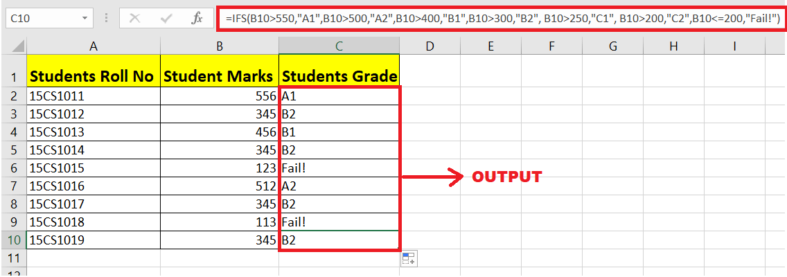
Eureka, without any hassle of nested IF, we fetched students’ grades as per the given grade score.
Explanation:
The IFS function checks the first condition – if 556>600, which turns TRUE; therefore, it returns grade A1. Again, for the following cell formula, the first test is evaluated s condition is found to be FALSE (345>600). It checks the following condition – if 345 > 500, which again evaluates FALSE. It moves to the next one- if 345> 400, when this condition is also found to be FALSE, it moves on to the next one to check – if 345> 300, this turns out to be TRUE it returns B2. Similarly, it evaluates the formula for all the cells and returns the Grade output.
Example 2 – Example to demonstrate that with IFS Function a default Value doesn’t exist.
In the above example, we have seen how the IFS function returns the perfect grade value for each cell as required but what if the test argument does not exist for any specified conditions?
For instance, let’s suppose in the above example only we have added one new row that contains Student Marks as 620; there is no test condition in this specified formula that matches this value. Therefore, this function will return the #N/A error.
Let’s look at this below.
Follow the below-given steps to run multiple tests and return a default value using the Excel IFS() function:
Step 1: Select a cell to calculate student’s Grade
Place your mouse cursor in the in the first cell of Score column so we can enter the formula and find the Grade for the specified marks as per the above score table. In our case, we have selected cell C2 of our Excel worksheet.
Refer to the given below image:
STEP 2: Enter the IFS function
To figure out the grade based on the grade chart. Start the formula using the equal to (=) sign followed by the built-in Excel IFS function.
STEP 3: Insert all the parameters
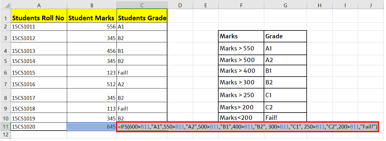
- Initially, you have to specify the first test parameter. Here, we will specify 600>marks,. The formula will be =IFS(600>B11,
- Next, we will specify the value parameter that will be returned if the above test parameter evaluates TRUE. The formula will be =IFS(600>B11,”A1″,
- Similarly, we will specify the subsequent test and value parameter to satisfy the further conditions.
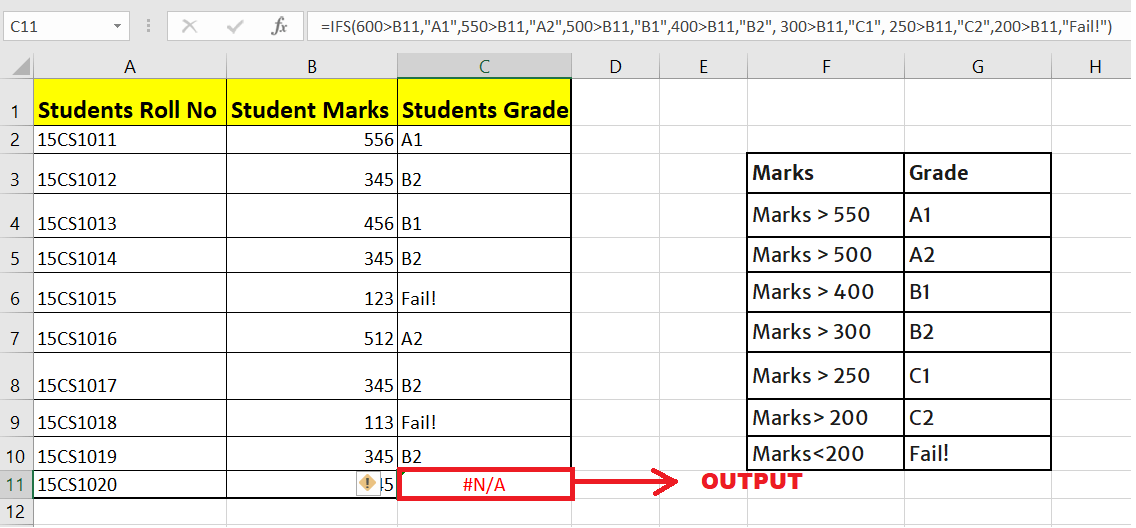
The overall formula becomes:
=IFS(600>B11,”A1″,550>B11,”A2″,500>B11,”B1″,400>B11,”B2″, 300>B11,”C1″, 250>B11,”C2″,200>B11,”Fail!”)
Step 4: The IFS function will return error
Since the value 645 falls under none of the given criteria, it should return the default function value as per the Excel formula rule. Since IFS does not have any default value, it returns the #N/A error.
Points to Remember
- The IFS function does not have any pre-defined default value that can be used when all the given conditions are not met.
- To supply a default value, enter TRUE as a final test, and a value to return when all the given conditions return FALSE.
- All the specified logical conditions must return either TRUE or FALSE. Any other output will force the IFS to return a #VALUE! error.
- If none of the specified conditions return TRUE, the IFS function will return the #N/A error.
Difference between IFS and Switch
Many of you might think that the IFS function works similarly to the SWITCH Function, but the Excel IFS function allows the user to test more than one condition in a single enclosed formula. Although both Switch and IFS functions are easy to write and understand when both are compiled with many conditions, they have their pros and cons. To understand their difference better, the following is the comparison table:
| S.NO | IFS | SWITCH |
|---|---|---|
| 1 | In IFS, you are required to repeat the expression in order to fetch the required result. | In Switch function, there is no need to repeat the expression as it required to be used just once in the function. |
| 2 | The Excel IFS function doesn’t accept any default value. | The Excel SWITCH function can accept a default value. |
| 3 | This function is not limited to exact matching. | This function is limited to exact matching |
| 4 | The IFS function requires expressions for each condition, so you can use logical operators as needed. | It is not possible to use operators like greater than (>) or less than (<) with the standard syntax |
IFS V/S Nested IF Statements
The Excel IFS function was introduced in MS Excel 2019. Before that, if users were compelled to use the nested IF statements. Though both the formulas work in the same manner the nested IF statements are much more complicated and are prone to errors when compared to the IFS function.
The only reason for this complication in nested IF functions is because formulas with nested IF use multiple parentheses and IF functions nested within one another, which is not the case with the IFS function. Therefore, the IFS function stands out and is the winner. Moreover, the syntax of IFS is relatively easier than nested IF and it is easy to understand.


