
Excel Highlight Cell Rules
Microsoft Excel pursuit is an indispensable part of every office. The biggest challenge Excel users face is all the cells in the spreadsheet look the same. The worksheet consisting of thousands of rows is formatted in the same boring pattern. The data in the cells are all different from the rest, so why is the appearance of each cell so identical?
Well, whenever there is a problem, Excel has a solution. The solution of Excel spreadsheets problem having identical cell appearance is Excel Highlight Cell Rules. Excel Conditional formatting permits the user to highlight cells with a specific color, depending on the value. This tutorial will discover how to highlight cells in an Excel worksheet using different examples.
What are Excel Highlight Cell Rules?
Excel Highlight Cell Rules is a premade feature of conditional formatting that enables the users to highlight cells or range of cells with a certain color, depending on your specified conditions.
Conditional formatting makes it easy to highlight cell values such as the user can easily identify the cells. It changes the appearance of a cell range based on specified conditions. The conditions are simple cell rules applied on numerical values, date values, identical string data, or duplicated and unique values. This feature assists the user in visually exploring and analyzing data, catching crucial matters, and highlighting important patterns and trends.
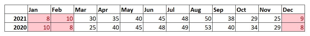
In the below example, we are given different Temperature data. Using Conditional Formatting Highlight Cell rules, we highlighted the cell containing the top 10% and bottom 10% values.
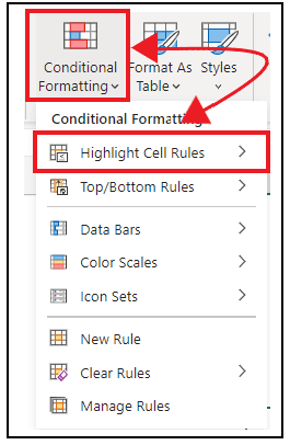
The Highlight Cells conditional formatting feature in Excel is found in the Conditional Formatting menu, typically listed in the ‘Styles’ group of the Home tab on the ribbon bar (refer to the below image).
Cell Rule Types

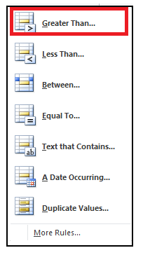
When you click on the ‘Conditional Formatting Highlight Cell Rules’ option, it further opens a window display six Highlight Cells Rules as given below:
- (>) Greater Than…
- (<) Less Than…
- Between…
- (=) Equal To…
- (ab) Text that contains…
- A Date Occurring…
- Duplicate/Unique Values…
Whenever the user selects any of the above six options, a dialog box appears, enabling the user to input a value or a cell reference to compare each cell’s value. If none of the above options fits your requirement, you can click on the ‘More Rules’ option and create your own highlight formatting rule. Using ‘More Rules’, you can create a condition to highlight cells containing unique data values.
Highlight Cell Appearance Options
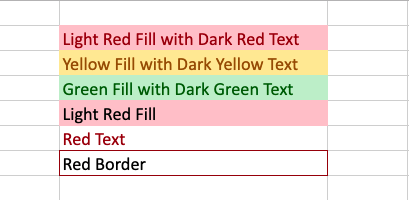
Microsoft Excel offers the pre-defined appearance options for conditionally formatting and highlighting the cells. The various options are as follows:
- Light Red Fill with Dark Red Text (default option)
- Yellow Fill with Dark Yellow Text
- Green Fill with Dark Green Text
- Light Red Fill
- Red Text
- Red Border
Example 1 – Excel Conditional Formatting Highlight Cell Rules Using Absolute Values
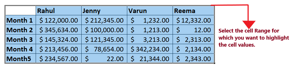
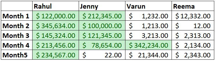
Below given is the monthly sales table. Apply Excel Conditional Formatting Highlight Cell Rules feature to your cells, and highlight cell value whose monthly sales value is greater than $ 300,000.00.
| Rahul | Jenny | Varun | Reema | |
|---|---|---|---|---|
| Month 1 | $ 122,000.00 | $ 212,345.00 | $ 1,232.00 | $ 12,332.00 |
| Month 2 | $ 345,634.00 | $ 100,000.00 | $ 1,213.00 | $ 12.00 |
| Month 3 | $ 145,324.00 | $ 121,345.00 | $ 3,213.00 | $ 2,313.00 |
| Month 4 | $ 213,456.00 | $ 78,654.00 | $ 342,234.00 | $ 2,134.00 |
| Month 5 | $ 234,567.00 | $ 22.00 | $ 21,344.00 | $ 2,343.00 |
Solution: Highlight Cell Rules is a feature Excel conditional formatting feature that quickly helps to format the selected cells based on their values. With the help of this example, we will cover the step-by-step procedure to implement it in our Excel worksheet.
Step 1: Select the cells or cell Range
The first step is to select the cells which you wish to format. In our case, we want to highlight the cells whose value is greater than 60. So we have selected the cell range from C3 to G8.
Refer to the below image:
Step 2: Click on Conditional Formatting Highlight Cell Rules
- Go to the Home tab of the Excel ribbon. Click on the Conditional Formatting listed in the Excel ‘Styles’ group.
- It will open the following options window; click on the Highlight Cells Rules option.
Step 3: Select the ‘Greater Than’ option
- As soon as you click on the Highlight Cell Rules, another secondary window appears, displaying the list of options.
- Since in the questions, it’s mentioned to highlight values Greater than 30000. So we will choose the Greater Than … option.
Refer to the below image.
Step 4: Enter the Value for which you want to apply the condition
- The Conditional Formatting ‘Greater Than’ dialog window will appear.
- In the ‘Format cells that are GREATER THAN:’ textbox, enter the input value 30000.
- Next, you will find a drop-down list on the right of the dialog box. It displays the pre-defined appearance format conditionally formatted cells. We have chosen the color option ‘Green Fill with Dark Green Text’ from the drop-down list.
- Once done, click on OK.
Refer to the below image:

Step 5: Excel will highlight the cells
As required, all the cells containing values greater than 30000 are highlighted with green fill with dark green text color.
Look out in the below given image for the resulting output:
Example 2 – Excel Conditional Formatting Highlight Cell Rules Using Cell References
Here, we have twisted a question a bit. Highlight the cells of your Monthly Sales Report table if the cell value is greater than the cell value for the previous month. We will use the same Excel table (refer to the above monthly sales report Excel Table).
Solution: The arrangement of the above question is quite tricky. Follow the step-by-step procedure to highlight the cell values greater than the cell value for the previous month:
Step 1: Select the cells or cell Range
- As per the above question, we have to apply cell formatting to the values in columns E-F-G (but not to column D because there is no previous monthly sales data to compare the values in column D).
- Select all the cells or Range of cell you wish to format. In our case, we have selected the cell range from E4 to G8.
Refer to the below image:

Step 2: Click on Conditional Formatting Highlight Cell Rules
- Go to the Home tab of the Excel ribbon. Click on the Conditional Formatting listed in the Excel ‘Styles’ group.
- It will open the following options window; click on the Highlight Cells Rules option.
Step 3: Select the ‘Greater Than’ option
- As soon as you click on the Highlight Cell Rules, another secondary window appears, displaying the list of options.
- Since in the questions, it’s mentioned to highlight cell value greater than the cell value for the previous month. So we will choose the Greater Than … option.
Refer to the below image.
Step 4: Enter the Value for which you want to apply the condition
1. The Conditional Formatting ‘Greater Than’ dialog window will appear.
2. In the ‘Format cells that are GREATER THAN:’ textbox, enter the cell reference A2. This can be specified by any of the following methods:
- Directly type the cell reference along with equal to symbol (=A2) in the input field.
Note: The equal to (‘=’) symbol is compulsory. If it is not used, Microsoft Excel will take the specified condition to be a comparison with the given text string “D4”)
or
- You will notice the
 symbol to the right of the textbox. Use your mouse cursor to click on the icon. It will take you to your Excel worksheet, click on cell D4.
Note: While using the second method to select the cell D4, Excel will convert the cell reference into an absolute reference – i.e. $A$2. You must to delete the $ signs for this specific example.
3. Next, you will find a drop-down list on the right of the dialog box. It displays the pre-defined appearance format conditionally formatted cells. We use the default color option ‘Light Red Fill with Dark Red Text’ from the drop-down list.
4. Once done, click on OK.
These above steps are shown in the below given image of the Conditional Formatting ‘GREATER THAN’ window:

Step 5: Excel will highlight the cells
In the given Monthly Sales Report Excel table, all the cells whose cell value is greater than the cell value for the previous month have been highlighted with the default ‘Light Red Fill with Dark Red Text’ color.
Look out in the below given image for the resulting output:

Eureka! We have covered all the step-by-step examples of Excel Conditional Formatting Highlight Cell Rules with this example. You are fully ready to try it out in your day-to-day Excel life.


