
Excel Floor Function
In your day-to-day Excel life, rounding is one of the most common operations performed while working with numbers. We all know rounding up or down a number is very helpful as it makes the calculation easier to estimate, communicate or work with. For example, you can round up a long decimal number to its nearest integer to report the output of complicated estimations.
This tutorial will cover the definition of Excel FLOOR Function, its syntax, parameters, return type, steps to implement FLOOR function in your worksheet, different examples to round decimal numbers to integers, round a number to nearest 5, and many more!
What is FLOOR Function?
The FLOOR function in Excel rounds down the specified number (in the number parameter) to the nearest provided multiple. FLOOR works like the MROUND function, but the advantage of using the FLOOR function is that it always rounds down.
This function rounds a number down to the specified multiple (provided in the Significance parameter). No rounding happens if the specified number is already an exact multiple, and this function returns the original number. The multiple to utilize for rounding any number is supplied as the significance parameter.
This function accepts two parameters, i.e., the number and the Significance. The Number argument represents the numeric value you want to round down to an exact multiple. The significance parameter represents the multiple to which the specified number should be rounded down. Although users commonly supply numeric values in the Significance parameter, time values can also be entered in the Significance text like “1:16”.
Note: The Excel FLOOR function is officially documented as compatibility function replaced by Excel FLOOR.MATH and FLOOR.PRECISE.
Syntax
Parameter
- Number (required)– This parameter represents the number that should be rounded.
- Significance (optional)– This parameter represents multiple to use when rounding. The sign much matches the number. So if the number is negative, the Significance must also be negative.
NOTE: In Excel 2003 & 2007 versions, it is mandatory that both the parameters (the number and significance) arguments must have identical signs; either both are positive or negative. Otherwise, an error is returned. But in the latest Excel versions, the FLOOR function has been enhanced, and it can hold a negative number and positive significance or vice-versa.
Return
The Excel FLOOR function returns a number rounding it down to a given multiple.
Rules for Excel FLOOR
The Excel FLOOR function performs rounding based on the following rules:
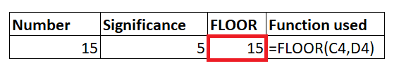
- If both the parameters are positive, the given number is rounded down towards 0. As you can see in the below image, the number argument is 6, whereas the significance is 5, so the number 19 is rounded to 15.

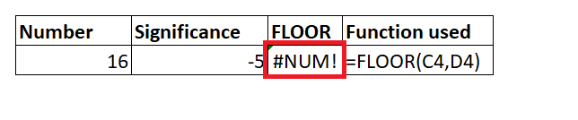
- If the parameter number is positive and the parameter significance is negative, the FLOOR function returns the #NUM error. Refer to the below image.
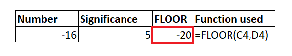
- If number is negative and significance is positive, the value is rounded down, away from zero. Refer to the below image.
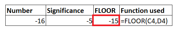
- If both the parameters are negative, the specified number is rounded up, toward zero. Refer to the below image.
- No rounding happens if the specified number is already an exact multiple, and this function returns the original number.
Examples
Example 1: Round down the given numbers to nearest 5
To round up the numbers to nearest 5 integer, follow the below given steps:
Step 1: Insert the helper columns
We will add the helper column helper with ‘Round up to 5’ in cell C3. In this column, we will use the FLOOR function to rounds the numbers down to a given multiple.
Refer to the given below image:

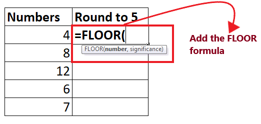
STEP 2: Implement the FLOOR Function
- Excel provides an inbuilt function FLOOR that helps to round a given number down, to the nearest multiple of a specified significance.
- In the “Round up to 5” helper column, start the formula with the equal sign (=) and type the FLOOR function. So our formula becomes: =FLOOR(
STEP 3: Insert the FLOOR Parameters
- At first it will ask for the number parameter. Here specify the number that you want to round of. In our case, we will refer to cell C3. So our formula becomes: =FLOOR (C3,

- Next, supply the significance parameter. In the question itself the significance is given as 5. So here we will pass 5. Therefore, our formula becomes: = FLOOR (C3, 5)

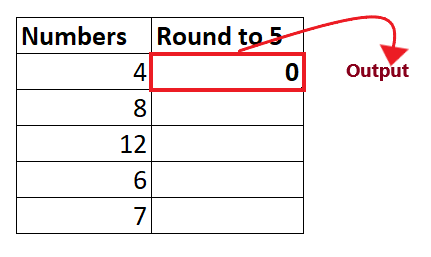
STEP 4: Excel will return the output
- Once you have typed the formula, press the Enter button to complete it.
- The above formula will return a number after rounding it down to 5. Since the given number is 5 will return 0 as output after rounding it down.
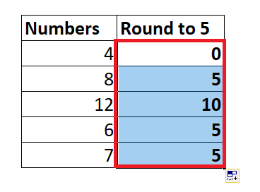
STEP 5: Copy the formula across all the cells
- Select the cell where you have typed the formula. Take your mouse cursor towards the end of the rectangular box. You will notice the cursor will change into a small thin black cross. Drag it over the cells you want to auto-fill.
- The formula will get copied where the absolute cell reference values will change and you will get the output for each cell.
You will have the following output.
Example 2: Round down the given pricing down to end with .99
You can also use the Excel FLOOR function to set the pricing after currency conversion, or getting discounts, etc. To round down the pricing to end with .99, follow the below-given steps:
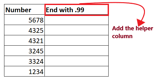
Step 1: Insert the helper columns
We will add the helper column helper with ‘End with .99’ in cell D3. In this column, we will use the FLOOR function to round down the pricing so it ends with .99.
Refer to the given below image:
STEP 2: Implement the FLOOR Function
- Excel provides an inbuilt function FLOOR that helps to round a given number down, to the nearest multiple of a specified significance.
- In the “‘End with .99′” helper column, start the formula with the equal sign (=) and type the FLOOR function. So our formula becomes: =FLOOR(

STEP 3: Insert the FLOOR Parameters
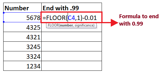
- At first it will ask for the number parameter. Here specify the number that you want to round of. In our case, we will refer to cell C3. So our formula becomes: =FLOOR (C4,
- Next, supply the significance parameter. In the question itself the significance is given as 1. So here we will pass 5. Therefore, our formula becomes: = FLOOR (C4, 1)
- Then subtract 1 cent, to return a price like 341.99, 54.99, 69.99, etc. Our formula becomes: =FLOOR(C4, 1) – 0.01
STEP 4: Excel will return the output
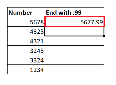
- Once, you have typed the formula, press the Enter button to complete it.
- The above formula will return a number ending with .99 after it rounding to 1. You will have the following output:
STEP 5: Copy the formula across all the cells
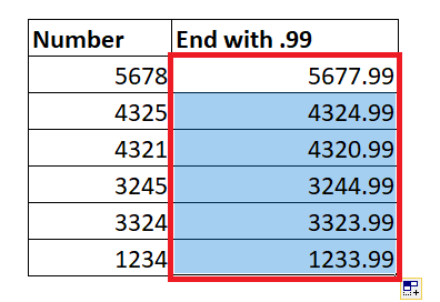
- Select the cell where you have typed the formula. Take your mouse cursor towards the end of the rectangular box. You will notice the cursor will change into a small thin black cross. Drag it over the cells you want to auto-fill.
- The formula will get copied where the absolute cell reference values will change and you will get the output for each cell.
You will have the following output.
Example 3: Round the different times in the Time column down to nearest 15 minutes
The Excel FLOOR function comprehends the time formats, and therefore can be used to round time down to the specified multiple. To round down the Time to nearest 15 minutes, follow the below given steps:
Step 1: Insert the helper columns
We will add the helper column helper with ‘nearest 15 minutes’ in cell D3. In this column, we will use the FLOOR function to round down the time to nearest 15 minutes.
Refer to the given below image:

STEP 2: Implement the FLOOR Function
- Excel provides an inbuilt function FLOOR that helps to round a given number down, to the nearest multiple of a specified significance.
- In the ‘nearest 15 minutes’ helper column, start the formula with the equal sign (=) and type the FLOOR function. So our formula becomes: =FLOOR(

STEP 3: Insert the FLOOR Parameters
- At first it will ask for the number parameter. Here specify the number that you want to round of. In our case, we will refer to cell C4. So our formula becomes: =FLOOR (C4,
- Next, supply the significance parameter. In the question itself the significance is given as nearest 15 minutes. Time values can also be entered in the Significance text like “1:16”. So here we will pass ‘0:15’. Therefore, our formula becomes: = FLOOR (C4, “0:15”)

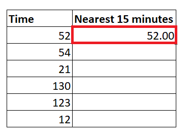
STEP 4: Excel will return the output
- Once, you have typed the formula, press the Enter button to complete it.
- The above formula will return a number after it rounding to “0:15”. You will have the following output:
STEP 5: Copy the formula across all the cells
- Select the cell where you have typed the formula. Take your mouse cursor towards the end of the rectangular box. You will notice the cursor will change into a small thin black cross. Drag it over the cells you want to auto-fill.
- The formula will get copied where the absolute cell reference values will change and you will get the output for each cell.
You will have the following output.

Other rounding functions in Excel
- You can implement the Excel ROUND function when you want to round the numbers normally.
- You can implement the Excel MROUND function when you want to round the numbers to the nearest multiple.
- You can implement the Excel ROUNDDOWN function when you want to round down to the nearest specified place.
- You can implement the Excel ROUNDUP function to round up to the nearest specified place.
- You can implement the Excel CEILING function to round up the given number to the nearest specified multiple.
- You can implement the Excel INT function to round down the given number and return an integer only.
- You can implement the Excel TRUNC function to truncate decimal places.


