
Excel Choose Function
The Excel CHOOSE function is one of those functions that may not seem useful on their own but is often merged with different other functions such as MATCH, INDEX, VLOOKUP to deliver several impressive benefits. The CHOOSE function returns a data or a reference from the predefined list of choices, by throwing the index of that value.
The function is available in almost all versions of excel starting from Excel 2007, Excel 2010, Excel 2013, Excel 2016, Excel 2019, and in the latest version, i.e., Excel 365.
Syntax
Parameters
- Index_number(required) – This parameter represents the position of the value that the function will return. You can pass any number between 1 and 254, a cell reference, or even type another formula in this argument.
- val1, val2, …– This parameter represents the list of options from which to choose. It can take up to 254 values. Though only the argument val1 is mandatory, and the rest all are optional. In this argument, you can pass number values, text values, excel cell references, and other
Excel CHOOSE function – 3 things to remember!
CHOOSE is a straightforward function, and if you know the syntax, you can implement it in your Excel worksheet without running into any errors. Though sometimes the output returned of the CHOOSE function is faulty or not the one you were expecting. The following pointer could be the reasons for an unexpected CHOOSE output:
- Limited Number values: The maximum number of values one can enter in the CHOOSE function is only 254.
- #VALUE! error: If the value passed in the ‘index_num’ argument is either less than 1 or greater than the total number of values present in the predefined list, Excel will throw the #VALUE! error.
- index_num is fractional value: If the value passed in the index_numargument is a fraction, it is round off to its lowest integer.
Example 1: Return values based on different conditions
One of the most usual tasks performed in Excel is to return different values based on various conditions. Though, users implement the conditional values by using Excel’s nested IF formula. But the CHOOSE formula is a good alternative to the nested IF formula; it is quick and easy.
Let’s understand the CHOOSE function with the help of some examples:
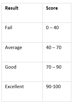
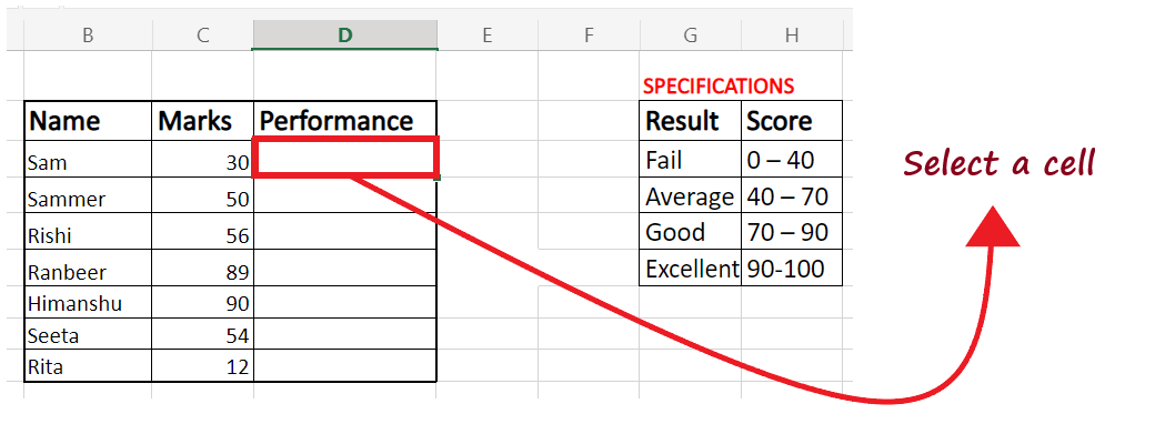
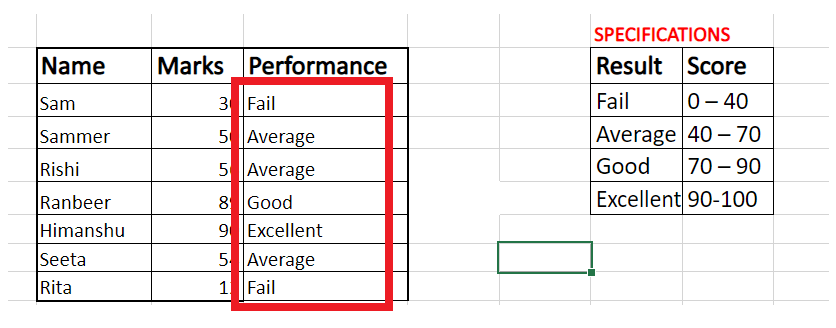
Let’s suppose you have an Excel list containing a student’s scores. You want to mark the performance of the students based on the below given conditions:
The first way to achieve this is by using the nested IF (nesting a few IF formulas inside each other) function.
=IF(B3> 90, “Excellent”, IF(B3>70, “Good”, IF(B3>=40, “Average”, “Poor”)))
The alternative of nested IFs is the CHOOSE formula. Follow the given steps to apply the CHOOSE function corresponding to the above condition:
1. Select a cell and start your formula by typing the equality sign (=).
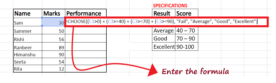
2. Enter the given Choose formula in the selected cell.
Formula used:
= CHOOSE ((B3>0) + (B3>=51) + (B3=101) + (B3>=151), “Poor”, “Satisfactory”, “Good”, “Excellent”)
3. Press the enter button, and Excel will choose data from the predefined list of values. As you can see in our case, the Marks are between 0-40 range, so it returned “Fail”.

4. For the next cells, drag the formula with the Fill handle. It will automatically copy the formula and change the cell reference for you.
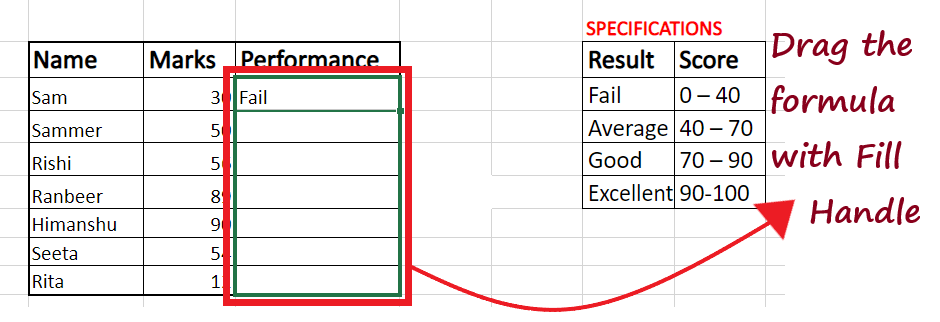
5. As shown below, you will have the performance categorization for each student.
How this formula works:
As we know that the choose formula takes two parameters here the first one is ‘index_num’. In this argument, we have passed all the conditions. Excel will evaluate all the conditions one by one and will return TRUE if any of the given conditions is met or it returns FALSE, if the conditions are not matched.
For instance, in the above formula we have applied four conditions. Out of which the first three conditions are met, giving us the following result:
=CHOOSE (TRUE + TRUE + TRUE + FALSE, “Poor”, “Satisfactory”, “Good”, “Excellent”)
Now, Excel will replace the TRUE with integer 1 and False with integer 0. Therefore, our formula will change and will give the following intermediate result:
=CHOOSE(1 + 1 + 1 + 0, “Poor”, “Satisfactory”, “Good”, “Excellent”)
After adding the values we will have:
=CHOOSE(3, “Poor”, “Satisfactory”, “Good”, “Excellent”)
That’s it, Excel will return the 3rd value from the specified list. In our case that is “Good”. Therefore the result is Good.
Example 2. Execute Choose function on the basis of different conditions
Let’s perform another example wherein we can use the Choose function and perform a series of calculations. In a similar method, you can use the Excel CHOOSE function to calculate a sales person’s commission based on their monthly sales.
In the below table we have listed two columns, where a commission amount of given to each seller based on their monthly sales:
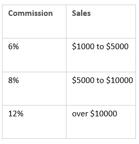
Based on the above specification we will write a formula where we will have 3 conditions (C3 > 0), (C3 >=5000), (C3>=10000) and in the next parameter passing the values. Therefore our formula will be as follows:
=CHOOSE ((C3>0) + (C3>=5000) + (C3>=10000), C3*6%, C3*8%, C3*12%)
It will evaluate the conditions and will return TRUE if the conditions are met.
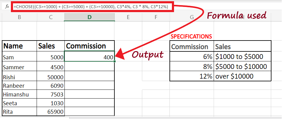
1. Select a cell and start your formula by typing the equality sign (=). Enter the given Choose formula in the selected cell.
Formula used:
=CHOOSE((C3>=1000) + (C3>=5000) + (C3>=10000), C3*4%, C3 * 8%, C3*12%)
2. Press the enter button, and Excel will choose data from the predefined list of values. Excel will calculate the commission based on their sales figure.
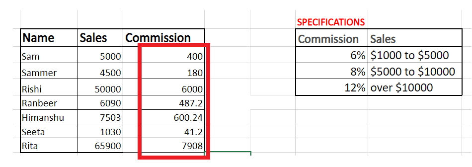
3. For the next cells, drag the formula with the Fill handle. It will automatically copy the formula and change the cell reference for you. You will have the following output.
Example 3: Excel CHOOSE formula to generate random values
Microsoft Excel provides various inbuilt functions, and one of them is the RANDBETWEEN function. This function is used to generate random integers in between the specified numbers (in bottom and top parameter). Apply the function in the index_num parameter of CHOOSE function, and Excel will generate random numbers for you.
For example, this formula can produce a list of random exam results:
=CHOOSE(RANDBETWEEN(1,3), “Lottery”, “Try Again”, “You Lose”)
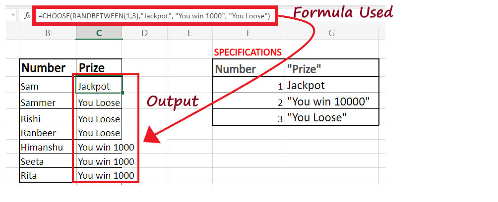
Although the explanation of the above formula is obvious, the RANDBETWEEN function will generate a random number from the specified top and bottom digits (1 to 3). Further, the CHOOSE function will return corresponding data from the given list of three values.
Note. RANDBETWEEN is a volatile function; therefore, if the user makes any changes to the excel worksheet, this function recalculates the values for every change and generates the data again.


