
What-if Analysis in Excel
In Excel, What-if analysis is a process of changing cells’ values to see how those changes will affect the worksheet’s outcome. You can use several different sets of values to explore all the different results in one or more formulas.
What-if Excel is used by almost every data analyst and especially middle to higher management professionals to make better, faster and more accurate decisions based on data. What-if analysis is useful in many situations, such as:
- You can propose different budgets based on revenue.
- You can predict the future values based on the given historical values.
- If you expect a certain value due to a formula, you can find different sets of input values that produce the desired result.
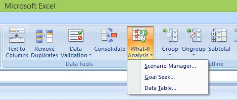
To enable the what-if analysis tool go to the Data menu tab and click on the What-If Analysis option under the Forecast section.

Now click on the What-If Analysis. Excel has the following What-if analysis tools that can be used based on the data analysis needs:
- Scenario Manager
- Goal Seek
- Data Tables
Data Tables and Scenarios take sets of input values and project forward to determine possible results. Goal seek differs from Data Tables and Scenarios in that it takes a result and projects backward to determine possible input values that produce that result.
1. Scenario Manager
A scenario is a set of values that Excel saves and can substitute automatically in cells on a worksheet. Below are the following key features, such as:
- You can create and save different groups of values on a worksheet and then switch to any of these new scenarios to view different results.
- A scenario can have multiple variables, but it can accommodate only up to 32 values.
- You can also create a scenario summary report, which combines all the scenarios on one worksheet. For example, you can create several different budget scenarios that compare various possible income levels and expenses, and then create a report that lets you compare the scenarios side-by-side.
- Scenario Manager is a dialog box that allows you to save the values as a scenario and name the scenario.
2. Goal Seek
Goal Seek is useful if you want to know the formula’s result but unsure what input value the formula needs to get that result. For example, if you want to borrow a loan and know the loan amount, tenure of loan and the EMI that you can pay, you can use Goal Seek to find the interest rate at which you can avail of the loan.
Goal Seek can be used only with one variable input value. If you have more than one variable for input values, you can use the Solver add-in.
3. Data Table
A Data Table is a range of cells where you can change values in some of the cells and answer different answers to a problem. For example, you might want to know how much loan you can afford for a home by analyzing different loan amounts and interest rates. You can put these different values and the PMT function in a Data Table and get the desired result.
A Data Table works only with one or two variables, but it can accept many different values for those variables.
What-If Analysis Scenario Manager
Scenario Manager is one of the What-if Analysis tools in Excel. Scenario Manager is useful in a case where you have more than two variables in the sensitivity analysis. Scenario Manager creates scenarios for each set of the input values for the variables under consideration. Scenarios help you to explore a set of possible outcomes, supporting the following:
- Varying as many as 32 input sets.
- Merging the scenarios from several different worksheets or workbooks.
If you want to analyze more than 32 input sets, and the values represent only one or two variables, you can use Data Tables.
Initial Values for Scenarios
Before you create several different scenarios, you need to define a set of initial values on which the scenarios will be based. Consider an example of a company that wants to buy Metals for their needs. Due to the scarcity of funds, the company wants to understand how much cost will happen for different buying possibilities.
In these cases, we can use the scenario manager for applying different scenarios to understand the results and make the decision accordingly. Now below are the following steps for setting up the initial values for Scenarios:
Step 1: Define the cells that contain the input values.
Step 2: Name the cells Metals_name and Cost.
Step 3: Define the cells that contain the results.
Step 4: Name the result cell Total_cost.
Step 5: place the formula in the result cell.
Step 6: Below is the created table.

To create an analysis report with Scenario Manager, follow the following steps, such as:
Step 1: Click the Data tab.
Step2: Go to the What-If Analysis button and click on the Scenario Manager from the dropdown list.

Step 3: Now a scenario manager dialog box appears, click on the Add button to create a scenario.

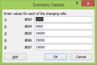
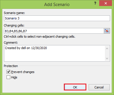
Step 4: Create the scenario, name the scenario, enter the value for each changing input cell for that scenario, and then click the Ok button.

Step 5: Now, B3, B4, B5, B6, and B7 appear in the cells box.
Step 6: Now, change the value of B3to 500 and click the Add button.
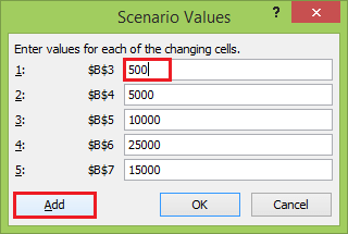
Step 7: After clicking on the Add button, the add scenario dialog box appears again.
- In the scenario name box, create scenario 2.
- Select the prevent changes.
- And click on the Ok

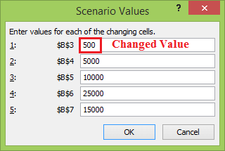
Step 8: Again appears scenario values box with the changed value of B3 cell.
Step 9: Change the value of B5 to 20000 and click the Ok button.

Step 10: Similarly, create Scenario 3 and click the Ok button.
Step 11: Again, appears scenario values box with a changed value of the B5 cell.

Step 12: Change the value of B7 to 10000 and click the Ok button.

The Scenario Manager Dialog box appears. In the box under Scenarios, You will find the names of all the scenarios that you have created.
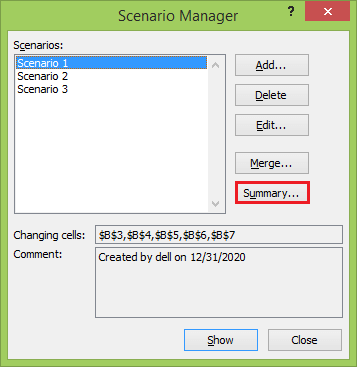
Step 13: Now, click on the Summary button. The Scenario Summary dialog box appears.
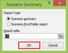
Excel provides two types of Scenario Summary reports:
- Scenario summary.
- Scenario PivotTable report.
Step 14: Select Scenario summary under Report type and click Ok. Scenario Summary report appears in a new worksheet. You will get the following Scenario summary report.

You can observe the following in the Scenario Summary report:
- Changing Cells: Enlists all the cells used as changing cells.
- Result Cells: Displays the result cell specified.
- Current Values: It is the first column and enlists the values of that scenario selected in the Scenario Manager Dialog box before creating the summary report.
- For all the scenarios you have created, the changing cells will be highlighted in gray.
- In the $C$9 row, the result values for each scenario will be displayed.
What-If Analysis Goal Seek
Goal Seek is a What-If Analysis tool that helps you to find the input value that results in a target value that you want. Goal Seek requires a formula that uses the input value to give the result in the target value. Then, by varying the formula’s input value, Goal Seek tries to solve the input value.
Goal Seek works only with one variable input value. If you have more than one input value to be determined, you have to use the Solver add-in. Below are the following steps to use the Goal Seek feature in Excel.
Step 1: On the Data tab, go What-If Analysis and click on the Goal Seek option.

Step 2: The Goal Seek dialog box appears.
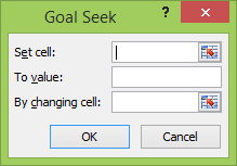
Step 3: Type C9 in the Set cell box. This box is the reference for the cell that contains the formula that you want to resolve.
Step 4: Type 57000 in the To value box. Here, you get the formula result.
Step 5: Type B9 in the By changing cell box. This box has the reference of the cell that contains the value you want to adjust.
Step 6: This cell that the formula must reference goal Seek changes in the cell that you specified in the Set cell box. Click Ok.

Step 7: Goal Seek box produces the following result.

As you can observe, Goal Seek found the solution using B9, and it returns 0 in the B9 cell because the target value and current value are the same.
What-If Analysis Data Tables
With a Data Table in Excel, you can easily vary one or two inputs and perform a What-if analysis. A Data Table is a range of cells where you can change values in some of the cells and answer different answers to a problem. There are two types of Data Tables, such as:
- One-variable data tables
- Two-variable data tables
If you have more than two variables in your analysis problem, you need to use the Excel Scenario Manager Tool.
One-variable Data Tables
A one-variable Data Table can be used to see how different values of one variable in one or more formulas will change those formulas’ results. In other words, with a one-variable Data Table, you can determine how changing one input changes any number of outputs. Below is an example of creating a one-variable data table.
A good example of a data table employs the PMT function with different loan amounts and interest rates to calculate the loan.
There is a loan of 1 00,000 for a tenure of 5 years. You want to know the monthly payments (EMI) for varied interest rates. You also want to know the amount of interest and Principal that is paid in the second year.
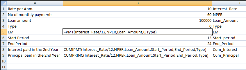
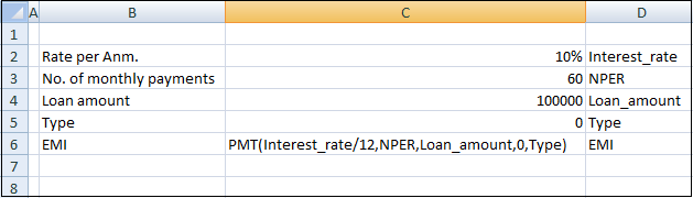
Step 1: Create the required table.
- Assume that the interest rate is 10%.
- List all the required values.
- Name the cells containing the values.
- Set the calculation for EMI, Cumulative Interest and Cumulative Principal with the Excel functions PMT, CUMIPMT and CUMPRINC, respectively.
- Below is the created table.
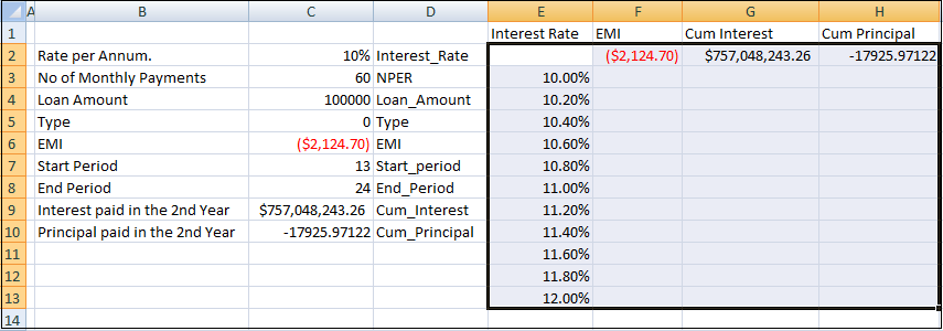
Step 2: Type the list of interest rate values that you want to substitute in the input cell.
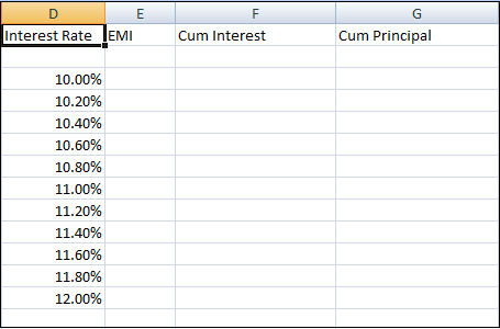
As you observe, there is an empty row above the Interest Rate values. This row is for the formulas.
Step 3: Type the first function (PMT) in the cell one row above and one cell to the right of the column of values. Type the other functions (CUMIPMT and CUMPRINC) in the cells to the first function’s right.
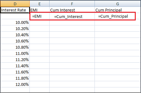
Step 4: The Data Table looks as given below.
Step 5: Select the range of cells that contains the formulas and values that you want to substitute, E2:H13.
Step 6: Go to the Data tab, select What-if Analysis and click on the Data Table tool in the dropdown list.
Step 7: Data Table dialog box appears.
- Click in the Column input cell box.
- And click on the Interest_Rate cell, which is C2.
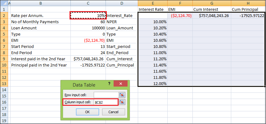
You can see that the Column input cell is taken as $C$2.
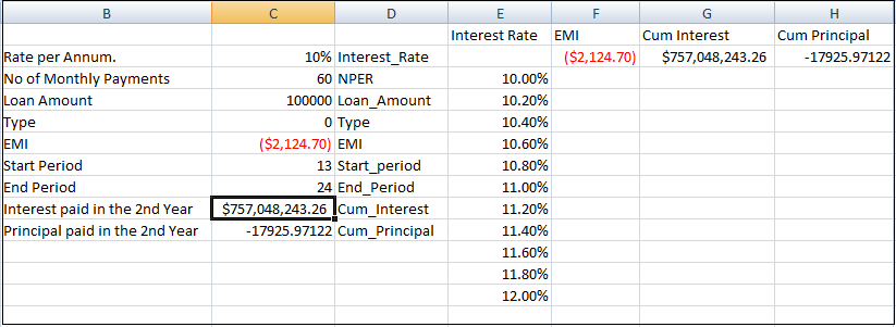
Step 8: Click on the Ok button.
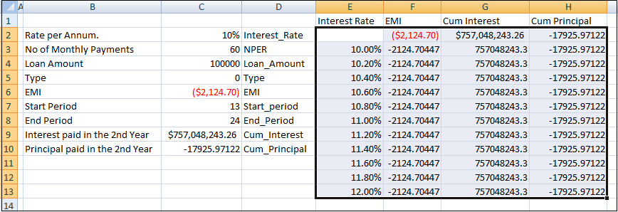
The Data Table is filled with the calculated results for each input value.
Two-variable Data Tables
A two-variable Data Table can be used to see how different values of two variables in a formula will change that formula’s results. In other words, with a two-variable Data Table, you can determine how changing two inputs changes a single output.
For example, a loan of 100000, and you want to know how different combinations of interest rates will affect the monthly payment.
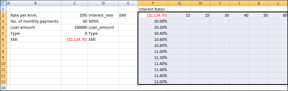
Step 1: Create the following table.
Step 2: Now create the Data Table
- Write =EMI in F2 cell.
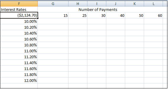
- Type the first list of input values, i.e., interest rates, down the column F, starting with the cell below the formula, i.e., F3.
- Type the second list of input values, i.e., number of payments across row 2, starting with the cell to the right of the formula, i.e., G2.
- The Data Table looks as follows.
Step 3: Select the range of cells that contains the formula and the two sets of values that you want to substitute, i.e., F2:L13.
Step 4: Go to the Data tab, click What-if Analysis and select Data Table from the dropdown list.
Step 5: Data Table dialog box appears.

Step 6: Click in the Row input cell box.
- Click on the NPER cell, which is C3.
- Again, click in the Column input cell box.
- Click the Interest_Rate cell, which is C2.

You will see that the Row input cell is taken as $C$3, and the Column input cell is taken as $C$2.
Step 7: Click on the Ok button.
The Data Table gets filled with the calculated results for each combination of the two input values.
Data Table Calculations
Data Tables are recalculated each time the worksheet containing them is recalculated, even if they have not changed.
To speed up the calculations in a worksheet that contains a Data Table, you need to change the calculation options to Automatically Recalculate the worksheet but not the Data Tables.


