How Insert Stiff Diagram in Excel
These are a few simple steps on how to create Stiff Diagram in Excel.
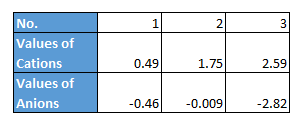
Step 1: Enter the values of cations and anions. Use the anion values in negative as shown below.

Step 2: Select 1, 3, and 5 (press Ctrl key, so select cells individually) and copy (Ctrl+c).

Step 3: Right click on empty cell -> Paste special -> Transpose

Step 4: Select the data in this table (2, 3, 4)

Step 5: Now go to Insert -> Charts -> Insert Scatter

Step 6: Now assign the data labels by the values in the first table. Select the blue dots by click -> right click -> format data labels.

Step 7: Select value from cells and then provide the range of cation names

Step 8: Format Data Labels -> Size and Properties -> Text Direction -> Rotate 90 degree

Step 9: Select free form diagram from Insert -> Shapes -> Freeform. Click on the dots to connect them into a shape as below.

Step 10: Remove the gridlines. Copy the chart and paste as an image. Then Format -> Rotate 90 degree.

To delete the point colors, right click on them and select color as white.
You can also add a horizontal axis to the chart by right click -> axes -> Primary horizontal axis.
Your Stiff Diagram is ready to use.
Template
Further reading:
Basic concepts
Getting started with Excel
Cell References


