Setting Cell Type and Font in Excel

MS Excel or Microsoft Excel is powerful spreadsheet software that allows users to record data in different cells across multiple worksheets. By default, Excel uses pre-defined formatting for each cell within the sheet, which can sometimes make it difficult to quickly read useful information from a related workbook with large amounts of data. However, we can adjust some basic formatting such as cell types and fonts in Excel to optimize the look and appearance of the workbook to some extent, highlight useful information to attract attention, and make the content easier to view and understand.

This article discusses the various ways to set a specific cell type and desired font for selected cells in Excel. By understanding these methods, we can easily apply number formatting to enter different types of data and change font style, size, color, etc.

Setting Cell Type

By setting a specific cell type in Excel, we typically specify the type of value or data that we want to enter for the corresponding cell. It is a method of choosing the format of how the values in corresponding cells are displayed. Excel allows users to enter or show different values like numbers, currency, dates, etc. However, the numerical values are the most commonly used data type in Excel cells.

There are multiple ways to access the supported cell type or formats in Excel, such as:

• After selecting the desired cell (s), we can go to the Home tab and click on the More icon from the bottom-right corner under the group named Number.
  
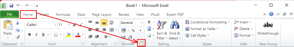
• We can select the cells to adjust the cell type of format, press the right-click button via the mouse, and choose the Format Cells option. After that, we need to click the Number tab.
  
• We can use the keyboard shortcut “Ctrl + 1” without quotes after selecting the respective cells and quickly access the Format Cells dialogue box. However, the key ‘1’ must be pressed from the keyboard area and not the number pad.
  

Note: To quickly adjust or choose a common cell type in Excel, we can go to the Home tab and select the desired one from the drop-down list under the category Number.

Supported Cell Type or Formats in Excel

The following are the built-in cell type of cell formats in Excel:

General

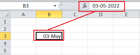
General is the default cell type or format for each cell in Excel. Whenever we type a number within the cell, Excel automatically identifies the format best suits the value entered. For example, if we type 3-5 in an Excel cell with default formatting, the value entered will change to a shorter date, i.e., 03-May. If we check the formula bar for the particular cell, the cell will display the given number (3-5) as 03/05/current year.

Number

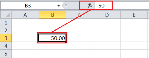
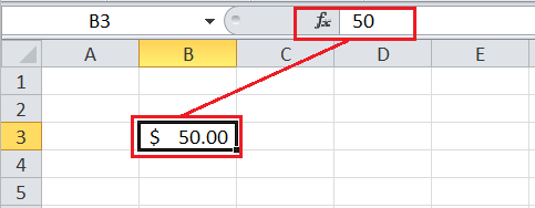
With a Number format in a cell, numeric values are displayed with decimal places, even if we do not manually type the decimal. For example, if we type 50 in a cell with a number format, the value (50) will change to 50.00. This particular cell type of number format displays numbers in a general form.

Currency

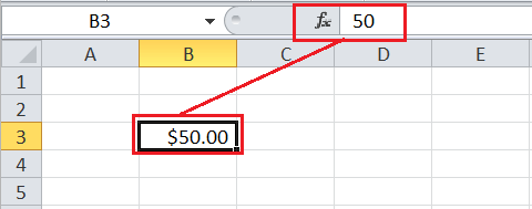
Setting the cell type as Currency, given values or numbers are displayed as currency with a currency symbol before the given values. The currency sign is added according to the chosen geographic location and can be changed as desired. For example, if we type 50 in a cell with currency format, the value (50) will change to $50.00. This cell type/ format is mainly used for general monetary values.

Accounting

The Accounting format is almost identical to the currency format and formats the given or entered numbers as monetary values. However, unlike the currency format, the accounting format aligns or lines up currency symbols and decimal points in a column. This cell type/format makes it easy to read long lists of currency figures.

Date

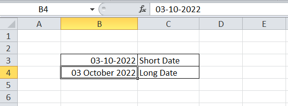
We can use this cell type in Excel to format given values as dates. Generally, short date and long date formats are used. Short format formats numbers as DD-MM-YYYY, while long date formats the numbers as DD MONTH YYYY. However, there are many other date formats that we can choose from the list accordingly.

Time

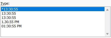
We can use this cell type (Time) in Excel to display given values as a time. It represents numbers as HH/MM/SS and adds AM (Ante Meridiem) or PM (Post Meridiem). There are many other pre-defined date formats in Excel, such as 1.30 PM, 13.30, etc.

Percentage

The Percentage cell type helps format the cell as a percentage with decimal places. Once formatted as a percentage, the decimal places, and the percentage (%) sign is automatically added with the entered value or number. For example, if we type 0.50 in a cell with a percentage format, the value (0.50) will change to 50.00%.

Fraction

The fraction values entered in Excel cells are converted as dates by default. For example, if we type 1/2 in an Excel cell with default formatting, it will automatically change to 01-Feb. The Fraction formats the given numbers or values as fractions and restricts the auto conversion of values into dates. It uses a forward slash and keeps the fraction values as they are supplied.

If a cell is formatted as a fraction, the entered value 1/2 will not be changed and appear as 1/2.

Scientific

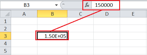
Setting the cell type as Scientific, Excel formats the corresponding cells in scientific notation (exponential form). For example, if we enter the value 1,50,000 in a cell formatted as Scientific, the value will change as 1.50E+05.

Besides, Excel automatically converts the entered value to scientific notation if it contains large integers. However, we can use the Number format to prevent Excel from converting large integers to scientific notation.

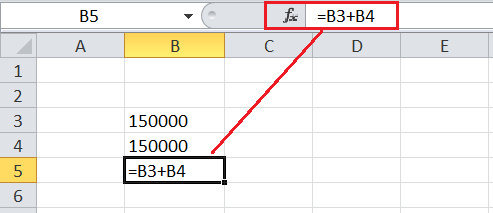
Text

Using the TEXT cell type, Excel formats the corresponding cell as normal text, which means that whatever we enter/type into the cell will appear the same as it was entered. By default, Excel uses this specific cell type when we type both text and numbers in the cell.

For example, if we enter a formula to add values from cells formatted as text only, we will not get results in mathematical form. The sum is not visible in the following image because the text values cannot be added together.

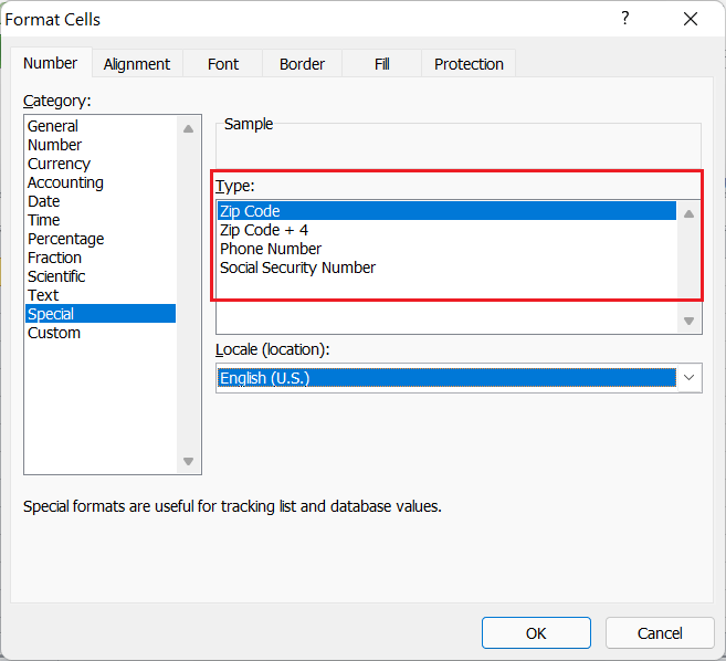
Special

As the name suggests, the Special cell type is used for numbers that require special formatting. We can enter numbers for ZIP codes, additional four-digit ZIP codes, telephone numbers, and Social Security numbers by special formatting. The particular cell type/format is also used to track the lists and database values.

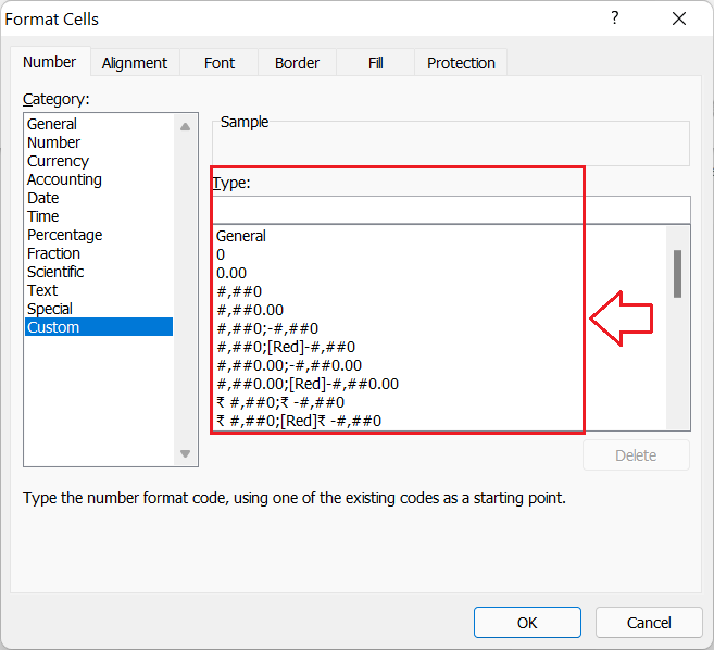
Custom

Although there are many pre-defined cell types in Excel, we can also create desired custom formats in selected cells. To create a specific format, we can go to Format Cells > Number Tab > Custom and enter the format code under the Type box.

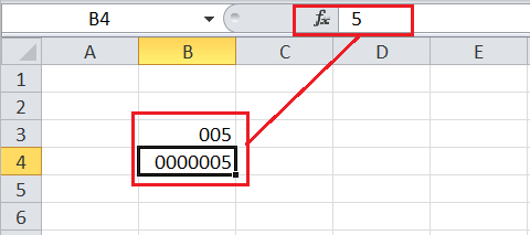
For example, when we enter numbers like 005 or 0000005 in cells with General formatting, the value entered is automatically changed to 5. However, by setting the custom number format, we can display the values exactly as they are entered. We can use the format codes 000 and 0000000 under the Custom Number Format box for the respective cells to display 005 and 0000005.

Setting Font

Excel has a variety of built-in customizations that can help us change the appearance of the sheet to a maximum extent. When setting fonts in Excel, we can change properties like font size, type, color, etc. Additionally, we can make the desired font bold, italic, or underlined.

The following are the two most common ways of the setting font within the Excel sheet:

• Setting Font from Ribbon
• Setting Font from Format Cells dialogue box

Setting Font from Ribbon

The ribbon is the main area where we can access most Excel tools or features. When setting font in Excel, we can use the ribbon options and adjust the desired font type, size, color, etc.

Changing Font Type

To change the font type or style in one or more Excel cells, we need to perform the following steps:

• First, we need to select the cell (s) consisting of the values we wish to format.
• Next, we need to go to the Home tab and click the initial drop-down list under the category font, as shown below:
  
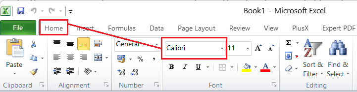
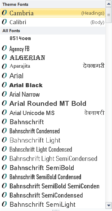
• We can scroll down to view all the installed fonts on our computer. We must click on the desired font type/style to instantly use it in the selected cell (s).
  

Changing Font Size

To change the font size in the desired Excel cells, we need to perform the following steps:

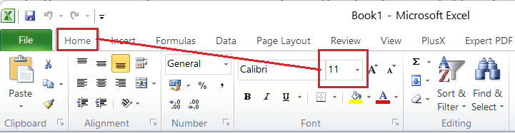
• First, we need to select the cells to adjust font size.
• Next, we need to go to the Home tab and click on the drop-down list associated with the number (i.e., 11, 12, etc.), next to the Font drop-down list, under the Category Fonts, as shown below:
  
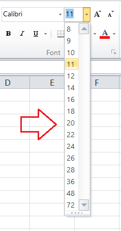
• There is a selection of multiple pre-defined font sizes to choose from. We can choose the desired font size by clicking the number from the list. However, if we don’t find a suitable size, we can type the number directly in the font size box and press the Enter key.
  
  Some font styles may have limited size options to keep them properly visible within the cells.
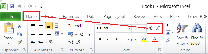
  Additionally, the font size can be quickly adjusted by clicking on Increase Font Size and Decrease Font size tools, displayed next to the Font size box.
  

Changing Font Color

To change the font color for the desired Excel cells, we need to perform the following steps:

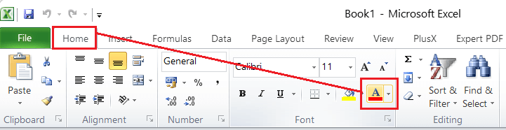
• First, we need to select Excel cells to apply the desired color.
• Next, we need to navigate the Home tab and click the last drop-down list under the category font. It is associated with the letter ‘A’ and a red color bar in its bottom, as shown below:
  
• After clicking the drop-down arrow for the font color, we can click on the desired color from the list of Theme Colors or the Standard Colors.
  
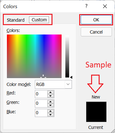
  If we don’t find the desired color, we can click the ‘More Colors’ option and choose any custom color from the Colors window. After selecting the color, we must click the OK button.
  

Note: If the cell is empty while setting the font in Excel, then as soon as we start typing text/data in the respective cell, the applied style, size, color, etc., will be applied automatically.

Setting Font to use Bold, Italic, and Underline

To change the font format in the desired Excel cell to make it bold, italic, or underlined, we need to perform the following steps:

• First, we must select one or more Excel cells to modify their respective values.
• Next, we need to go to the Home tab and click the Bold (B), Italic (I), or Underline (U) shortcut under the category Font. These tools help to change the appearance of the selected cell accordingly.
  
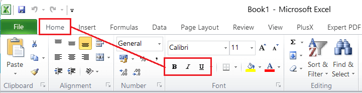
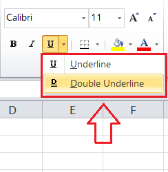
  To choose between single and double underlines, we can click on the drop-down arrow next to the Underline (U) shortcut.
  

Setting Font from Format Cells dialogue box

Setting the font from the Format Cells dialogue box is another straightforward method in Excel. To access the Format Cells dialog box, we can use the keyboard shortcut ‘Ctrl + 1’. Since we need to adjust the font, we have first to select the cells to format and then go to the Font tab from the Format Cells dialog box. It will look like this:

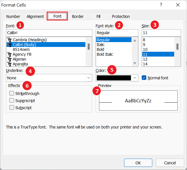
In the above dialogue box, we can modify the font in various ways using different sections, such as:

1. This section helps us to select the desired font installed on our computer. We can scroll drop the list to view more fonts.
2. This section helps us choose the desired font style: regular, bold, italic, and bold italic.
3. This section helps us to set the desired font size. We can also type the desired value for font size in the box.
4. This section helps us insert or add an underline below the values in cells.
5. This section helps us choose the desired color for the text/ values in cells.
6. This section helps us select different font effects, such as Strikethrough, Superscript, and Subscript. We can select the respective checkbox to apply the specific effect.
7. This section displays the preview of the font as per our applied settings. We can ensure that the font is adjusted as desired without having to apply the corresponding settings to the parent cells.

After adjusting the font properties, we need to click on the OK button, and the same properties will be immediately applied to the selected cells within the sheet.

Important Points to Remember

• Excel allows users to format data and time simultaneously.
• It is important to note that the font color should not be the same as the cell background color; otherwise, the corresponding font value will not be visible or will become invisible.
• When we want to change the font’s appearance to bold, italic or underlined, we can also use the keyboard shortcut ‘Ctrl + B’, ‘Ctrl + I’ and ‘Ctrl + U’, respectively.
• The Format Painter tool helps to copy one cell format to another.
• We must select the desired cells before formatting cells or fonts in Excel. When selecting multiple cells, we must click on respective cells while holding the Ctrl (for non-continuous cells) or Shift (for contiguous cells) key.

---