
Pie Chart In Excel
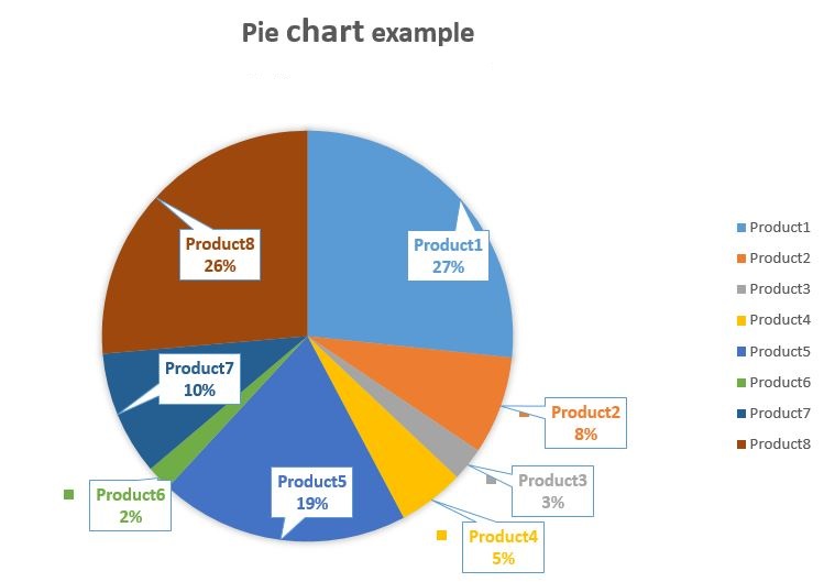
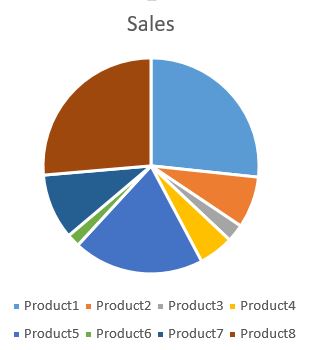
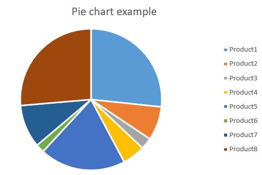
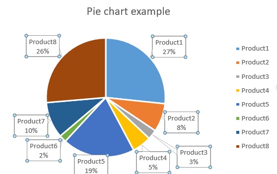
A pie chart is often used at home, office and business. Its popularity comes mainly from the transparency of the presented data. A pie chart is best suited to show the data as part of a whole. For example data about sales you can create pie chart like this:
Let’s see how to create such pie plot.
How to insert Pie Chart?
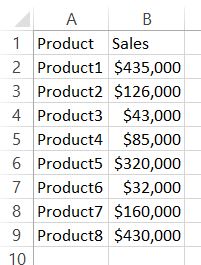
You have already learned how to create a chart in Excel. A pie chart is created the same way as any other type. Action starts with the selection of data. First prepare a table with data.
Then go to the Insert tab in the ribbon Excel. Find and select the Charts section -> Pie. You will insert a pie chart.
The question is which one to choose.
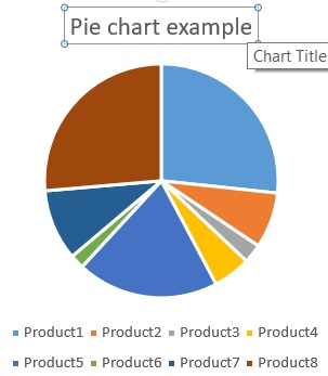
Pie Chart will look like this:
This one is the most basic one. I like it and would choose it for sure.
3D Pie Chart
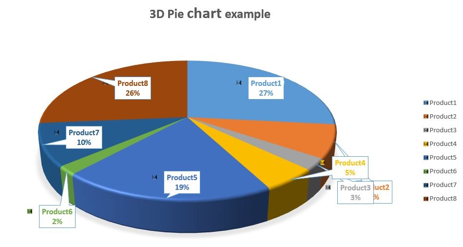
You may say it looks better but I don’t like anyway. The main reason is that the front pie does not look properly. Blue pie looks bigger then brown one but it is not (19% is much less than 26%).
Bar of Pie chart

This one you may consider to choose when there are a few dominating values and many of others which you don’t care so much.
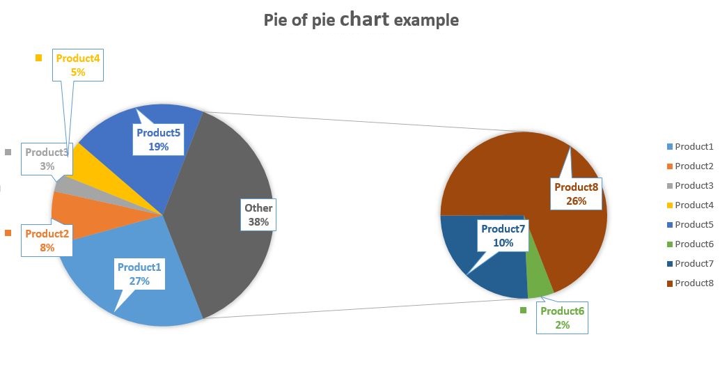
There is also a possibility to create multi level pie chart.
Basically pie of pie is very similar to bar of pie. You may choose the one you like more. Functionally they do the same.
Doughnut chart
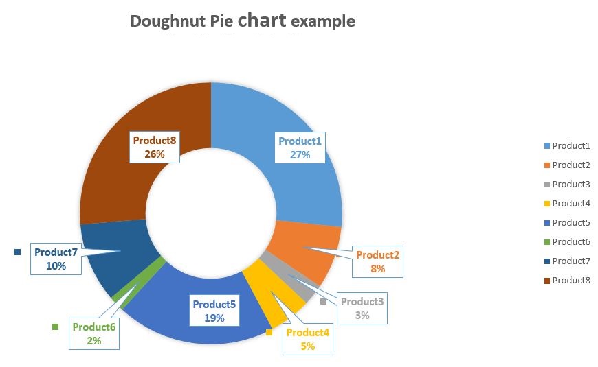
You can consider this one having many series of data or when you like sweets so much. This type is not so popular as pie chart.
Let’s choose regular pie chart as an example an follow on this one as an example. At the beginning it does look like that.
At the beginning let’s change chart title. It is simple. You just need to edit text field of chart.
Pie chart formatting
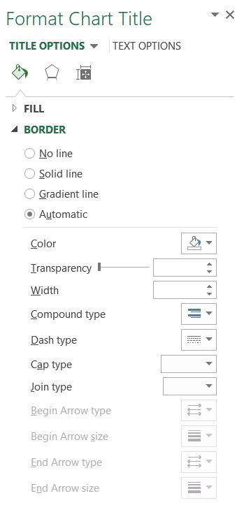
Right click the chart title and choose Format Chart Title. New menu on the right side of the screen pops. It gives you more opportunities to format chart title.
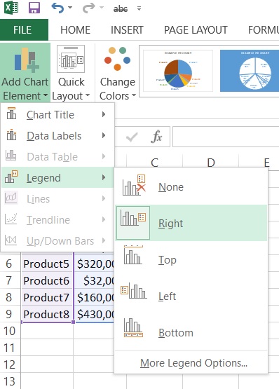
The next thing I’d like to format is chart legend. I don’t like it on the bottom because it is decreasing the pie. I’d move it on a side. There is a dedicated option for that in ribbon menu.
Pie plot became bigger thanks to that. As we all know the size matters.
There are much more formatting options available. Just once click your legend to open formatting menu on the right side of the screen. The same as you did before for chart title.

Where are data labels? It’s a high time to add them. You already know where you can find it in ribbon menu.
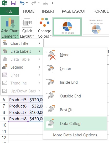
Only 3 of them are worth to consider:
- Outside End
- Best Fit
- Data Callout
I decided to choose Data Callout.
They did not fit perfectly. I customized two of them by simply moving them with my mouse. Now I can see every of them clearly. They do not overlap. That’s the most important thing.
However to increase the visibility even more you can manually remove irrelevant labels with DELETE keyboard button.

I’ve deleted two labels which I did not care too much. Pie chart looks much better now.
For further tweakings there is a bunch of additional formatting options available for you.

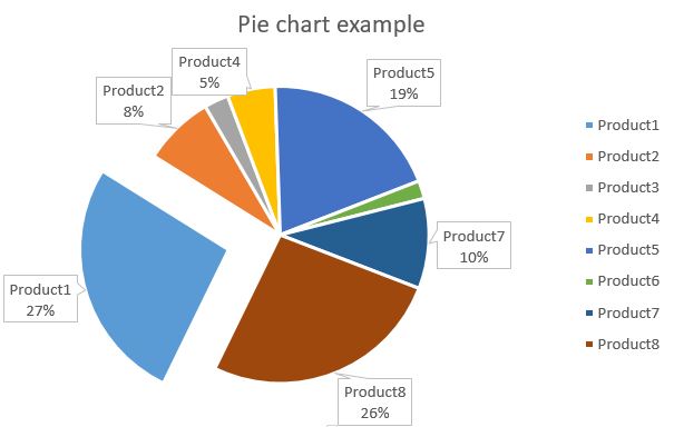
Suppose Product1 is the most important value in our chart. Then you have to show that. Double click Product1 slice to open Format Data Point menu.

I have changed the angle of first slice and exploded the data point. Here you can read more on how to explode pie slices.
Now I can see the most important part of the chart clearly.
This is how to insert and format pie plot in Excel. Still not enough? Check more pie chart tips and tricks we prepared for you.
Template
Further reading:
creating dynamic chart title from a cell
Two chart types in one chart
Pivot chart
Basic concepts
Getting started with Excel
Cell References


