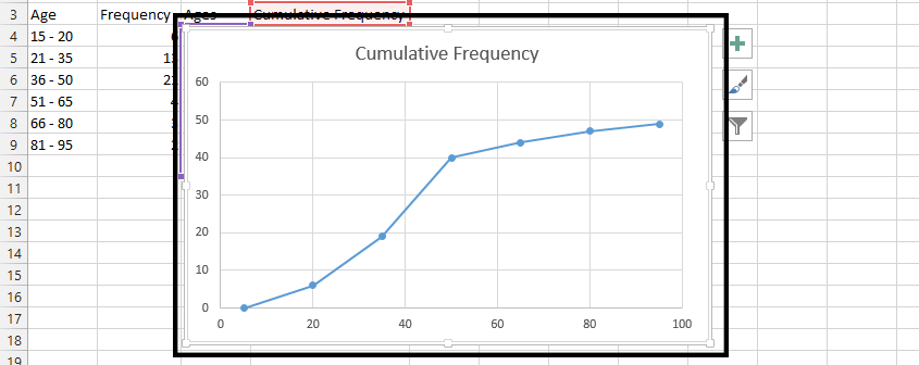
Ogive Charts In Excel
 1. Write ages on an empty column (1), and write the last numbers in the ages (2).
2. On an empty column, write Cumulative Frequency
3. Click under the Cumulative Frequency, and type =B4, which is the value under Frequency in column B.

4. Click under the result from previous result (1), and type =B5+B4.

Note: Follow this step on the rest, by typing
- =SUM(B6: B4 beside 50,
- =SUM(B7:B4) beside 65,
- =SUM(B8:B4) beside 80, and
- =SUM(B9:B4) beside 95.
5. Choose two cells under ages and cumulative frequency, right click on them (1), and choose insert (2).

6. Choose shift cells down (1), and press ok (2).

7. Put 0 under the cumulative frequency (1), and choose a number that rhymes with the ages under ages (2).
Note: We choose 5, because it makes it rhymes with the rest of numbers in the same column.
8. Highlight all the rows in both ages and cumulative frequency.

9. Click insert (1), choose scatter chart (2), and choose scatter chart with marker (3).

In conclusion, we have created a chart that looks like this:

Template
Further reading:
Basic concepts
Getting started with Excel
Cell References


