How to use the IF function in Excel
IF function is the most commonly used, simple, in-built, easy-to-use, and popular Microsoft Excel function. IF function is also known as logical tests because it is used to test a logical condition. It allows you to perform the comparisons between two values and returns results in one value, either TRUE or FALSE. For example, if you want to pass the exam, then score marks above 60. =IF(marks>60,”Pass”,”Fail”).
Syntax for IF function
We use the below syntax to use IF function in Microsoft Excel document –
The IF function contains 3 bits of information that is:
logical_test – It is a logical expression that is used to evaluate as TRUE or FALSE.
value_if_true – It returns TRUE when logical_text evaluates.
value_if_false – It returns FALSE when logical_text evaluates.
IF function is applied to Microsoft Office 365, Excel 2019, Excel 2016, Excel 2013, Excel 2011 (for Mac), Excel 2010, Excel 2007, Excel 2003, Excel 2007, as well as Excel XP.
1. Simple IF Function
Simple IF function directly checks condition if the condition is met with the requirement, then IF function returns TRUE, otherwise returns FALSE.
Steps to Use Simple IF Function
Follow the below steps to use the Simple IF function in Excel document –
Step 1: Open a Microsoft Excel document by double-clicking the Microsoft Excel icon on the Desktop.
Note: To open new Excel document click File -> New -> Blank document -> Create. To open an existing document click on the File -> Open -> Browse desired document location -> click Open button.
Step 2: Type your desired data on the Excel document.
Note: If you open an existing document, then skip Step 2.
Step 3: Place the cursor point on the cell where you want to display the IF function result. (In our case, we use cell B2 to display the results).
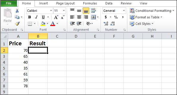
Step 4: In the desired cell, type =IF(A2>60,”Pass”,”Fail”) to check the IF condition.

Note: In our case, if marks obtained by students are greater than 60, then the IF function returns pass, else it returns fail.
Step 5: Press the Enter key from the keyboard to view the result.
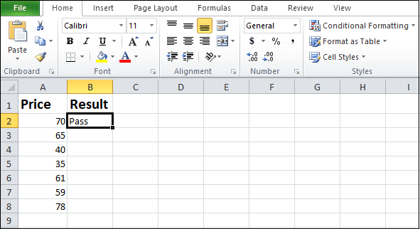
Note: In our case, 70>60, so the result is Pass.
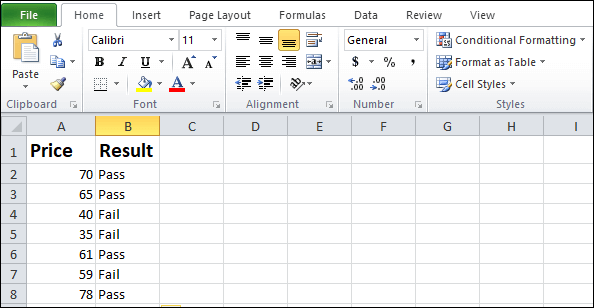
Step 6: Click on the small black dot and drag it at the end of the cell containing the values. See the below screenshot.

Microsoft Excel will automatically calculate Result (Pass or Fail) for the remaining cells, as shown in the below given screenshot.
Nested IF function
IF statement inside another IF or else if statement is called the Nested IF function. This function is used when you need to test more than one (multiple) conditions.
Syntax for Nested IF function
The below syntax is used for the Nested IF function –
Nested IF function example in Excel
Let’s see the below example to use the Nested IF function in Microsoft Excel document –
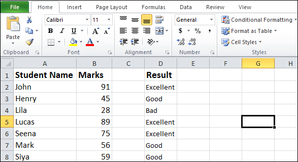
In our case, If marks obtained by a student is greater than or equal to 75 then the result will Excellent, else if marks obtained by a student is greater than or equal to 60, the result will be Very Good, else if marks obtained by a student is greater or equal to 40, the result will be Good, else the result will be Bad.
Steps for Nested IF function
Step 1: Double click on the Microsoft Excel icon to open a Microsoft Excel document.
Step 2: Type or prepare a list of data in the Microsoft Excel document.
Step 3: Place the mouse pointer in your desired cell where you want to display the result.
Note: In our case, D2 is used to view the result.
Step 4: Type formula =IF(B2>=75,”Excellent”,IF(B2>=60,”Very Good”,IF(B2>=40,”Good”,IF(B2>=10,”Bad”)))) in your selected cell of the Microsoft Excel document.

Step 5: Press the Enter key from the keyboard after completing the formula. The result will appear in your desired cell.
Step 6: Click on the small black square box and drag it at the end of the cell that contains data. See the screenshot.

Now, The Microsoft Excel will automatically calculate result for the remaining cells as shown in the screenshot given below.
IF function with OR/AND conditions
Microsoft Excel also allows us to use the IF function with the combination of both OR as well as AND functions.
Example 1 – IF function with AND
AND function returns TRUE if both conditions are satisfied. Otherwise, it returns FALSE.
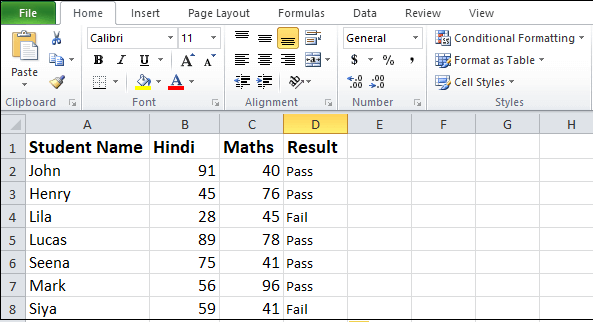
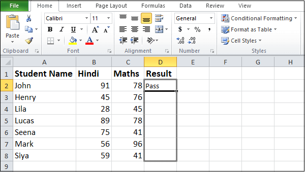
In this example, If marks obtained by a student in Hindi is greater than 60 and marks obtained by a student in Math is greater than 70, then AND function return PASS otherwise returns FAIL.
Below steps shows the result of the IF function with AND –
Step 1: Open a new or an existing Microsoft Excel document where you want to apply the IF function with AND.
Step 2: Prepare a document based on your requirement.
Step 3: Place the cursor on the cell where you want a result to display.
Note: In our case, we use cell D2 to display the result.
Step 4: Type or copy paste the formula =IF(AND(B2>=60,C2>70),”Pass”,”Fail”) in your selected cell.

Step 5: Once the formula is completed, press the Enter key from the keyboard.
Step 6: If both conditions are satisfied, then the result “Pass” will appear on the screen.

Step 7: Click on the small black square box and drag it at the end of the cell that contains data. See the screenshot.
Now, Microsoft Excel will automatically calculate a result for the remaining cells, as shown in the screenshot given below.

Example 2: IF function with OR
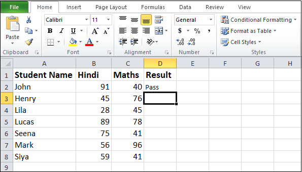
OR function returns TRUE if atleast one condition is satisfied. Otherwise, it returns FALSE.
The below steps will show the result of the IF function with OR.
Step 1: Open a new or an existing Microsoft Excel document where you want to apply the IF function with OR.
Step 2: Prepare a document based on your requirement.
Step 3: Place the cursor on the cell where you want a result to be displayed.
Note: In our case, we use cell D2 to display the result.
Step 4: Type or copy paste the formula =IF(OR(B2>=60,C2>70),”Pass”,”Fail”) in your selected cell.

Step 5: Once the formula is completed, press the Enter key from the keyboard.
Step 6: If atleast one condition is satisfied, then the result “Pass” will appear on the screen.
Step 7: Click on the small black square box and drag it at the end of the cell that contains data. See the screenshot.

Now, Microsoft Excel will automatically calculate the result for the remaining cells, as shown in the screenshot given below.