
How to define custom rules for conditional formatting in Excel?
Excel allows users to define their own custom rules/conditions of conditional formatting to format the cells data. These new customized rules help the users to format and highlight the data according to them. However, conditional formatting offers several pre-set conditions.
“Custom rules need to be defined when pre-set conditions do not have such rules.“
The custom rules of conditional formatting are new rules whose definition is not present in pre-set conditions. It means that – a user needs to define when it’s not available in pre-set conditions. Otherwise, the user can choose the preferred condition to format or highlight the Excel table data.
When setting new rules for custom conditions, you need to write the required formula to apply the customized conditional formatting on the selected data.
Why need to define custom rules?
If no option satisfies the criteria you are looking for in the pre-set conditions, you can define your own custom rules to format the cell’s data. For which, you need to write a formula while creating a custom rule to set criteria on the selected data.
- If the data match with the defined criteria, selected cells will be highlighted. Otherwise, they will remain the same.
- The custom rule helps the users to format the cells accordingly by defining their own rules.
Where to set new custom rules?
Here, we have steps to create custom rules for conditional formatting and an example to apply that custom rule on the targeted data. You can define new custom conditions in Excel to set user-defined rules.
Following is the location from where you can set the new rules of conditional formatting.
In the Home tab, go to the Conditional Formatting > New Rule.

Select a rule type from the opened panel. For defining the custom condition, click on the last option “Use a formula to determine which cells to format“.

From here, you can set custom rules. Now, let’s understand with an example.
For example –
For the row-to-row comparison of two columns, there is no predefined conditional formatting rule. So, we will define a custom rule for this and highlight the cell if matches are found; otherwise, not.
Steps to set new rules
Following are the steps to define custom rules (new rules) in Excel to format the cell data:
Step 1: We have this dataset for comparison. Select the row which you want to check the values are same or not.

Here, we can easily compare for simple data only by seeing the data. But for complex data, it is not easy to match the values.
Step 2: Now, under the Home tab, go to Conditional Formatting > New Rule.

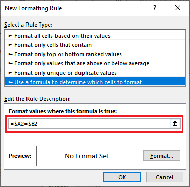
Step 3: Here, click on the last option Use a formula to determine which cell to format from the rule type list to choose rule type.

Step 4: Here, inside the formula field, specify the cells you want to compare in the following format, e.g., =$A2=$B2 for the second row.
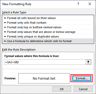
Step 5: In the end, specify the format for matched cell by clicking on the Format button and see the preview of it inside the Preview box.
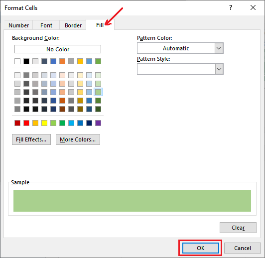
Step 6:
- Here, navigate to the Fill
- Choose a background color to highlight the matches.
- Click the OK
Step 7: See the preview in the preview section of that how row looks like if a match is found. After finalizing all the things, click the OK button and save all changes.

Step 8: You will see that row has not been highlighted because the A2 and B2 do not contain the exact same values.

Step 9: By following the same steps, compare the next row data. See that everything is set up successfully. Now, click the OK button to get the result.

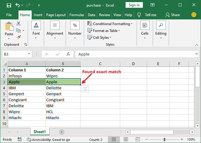
Step 10: Look at the following screenshot, that the 3rd row has been highlighted because it gets the same data in both columns.
Step 11: Similarly, we will check for all rows one-by-by present here.
After comparing both columns, see the Excel worksheet that the rows having the same data in both columns have been highlighted and remains are as they are without highlighting.

It will highlight all the matching data rows in the format you have chosen previously. Like this, we can define the custom conditions in conditional formatting.


