How to create a drop-down list in Excel

MS Excel or Microsoft Excel is currently the most powerful spreadsheet software with various versions with distinctive features and works in offline and online modes. It enables users to record large amounts of data within cells in different worksheets of a workbook. When dealing with massive data sets in Excel, we always focus on simplifying our work, reducing time, and maintaining the accuracy of the data. A drop-down list is one such element in Excel that comes in handy for meeting our needs, saving time in inputting information while eliminating the possibility of errors.

In this tutorial, we discuss the various step-by-step methods to create a drop-down list in an Excel worksheet. Before we move on to the methods, let us introduce the drop-down feature/tool in Excel.

What is Drop-Down List in Excel?

Excel’s drop-down list refers to a pre-defined list of various items that enable users to select any desired item as input data quickly. Drop-down lists prevent the insertion of data other than the ones in the list. Thus, it restricts the typing of manual data entries, reducing the chances of misspellings, incorrect data input, and the occurrence of garbage values in the cell.

Drop-down lists are commonly used on many websites or applications that accept data from users. Similarly, we use them in excel sheets so that users can fill in form details or provide/select other data types. Also, the drop-down lists are user-friendly, easy to use, and attractive.

For example, the following sheet shows a simple drop-down list that only accepts user input as ‘yes’ and ‘no’. Users do not have the option to type anything but only choose between these two listed options. Using a drop-down list ensures that the input is correct and to the point.

Steps to create a drop-down list in Excel

There are several methods in Excel to help us create drop-down lists in our worksheets. However, the most common method to insert or create drop-down lists involves using Excel’s ‘Data Validation’ tool/feature. Other methods include using a ‘Form Control’ combo box and an ‘ActiveX Control’ combo box. But, they are comparatively complex.

Let us now discuss the creation of different types of drop-down lists using the ‘Data Validation’ tool:

Creating a Static Drop-Down List

When we create a static drop-down list in Excel, our drop-down list does not update based on the newly added item at the end of the given range. This means no new entries will be added to the drop-down list created, even if we include them in the source data range. Lists and their items will remain static or fixed until we edit the entire drop-down list via Data Validation rules. However, we can add items in the static drop-down list by inserting the item (s) in the middle of the range.

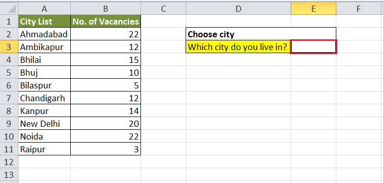
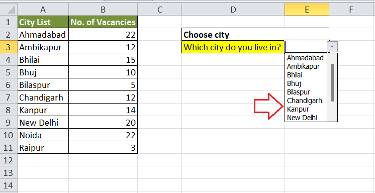
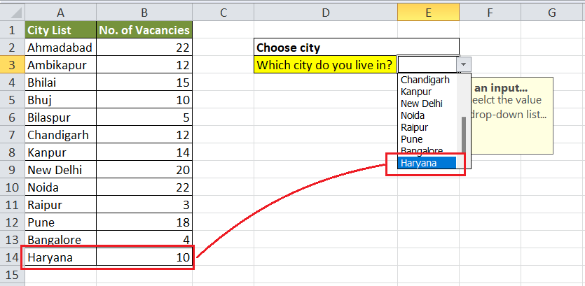
Consider the following tables as an example data set where we have some names of cities in column A, and the next column B contains the number of vacancies available in the respective cities. Suppose we want to create a drop-down list of given cities in cell E3, as shown below:

To create a static drop-down list like in the above image, we need to perform the following steps:

• First, we need to select a cell where we need to insert or create a drop-down list. In our case, we select cell E3.
  
• After selecting the effective cell, we need to navigate the Data tab > Data Validation > Data Validation.
  
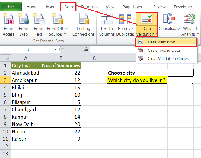
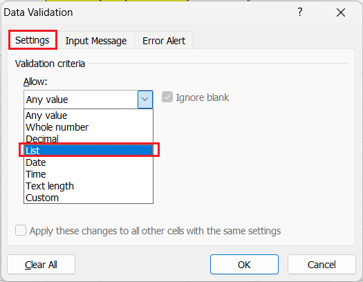
  Additionally, we can access the ‘Data Validation’ using the keyboard shortcut ‘Alt + A + V + V‘.
• In the Data Validation window, we must select the ‘Settings‘ tab. After that, we must select the ‘List’ option from the drop-down list under the ‘Allow‘ section, as shown below:
  
• Once we select the ‘List’ option, we see a box associated with the ‘Source‘ option to provide items for a drop-down list. We can either type the item names divided by Commas or select the range of cells from the sheet. All the selected items or typed values will be displayed in a drop-down list. In our case, we select a range A2:A11.
  
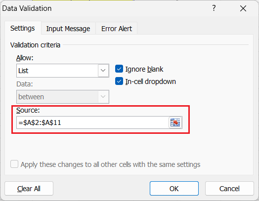
• Lastly, we must click the OK button, and our drop-down list will be immediately created in the selected cell.
  
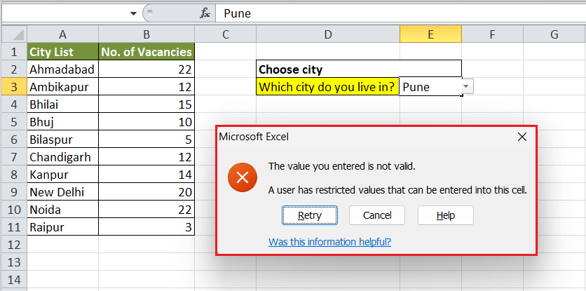
  If we try to manually enter any value in a cell with a drop-down list, we will get an error message, as shown below:
  
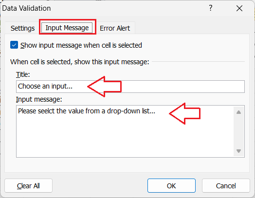
  The message displayed in the above image can also be modified accordingly, as discussed in the subsequent steps.
• We need to insert the input message or Error alert message while creating a drop-down list via the Data Validation window. Since we have already created a drop-down list, we must edit it and insert the input message and error alert accordingly. So, we use the keyboard shortcut ‘Alt + A + V + V’ to open the ‘Data Validation’ window.
  
• In the Data Validation window, we need to go to the ‘Input Message’ tab to type a message we want to display when the corresponding cell is selected. We can type or enter any ‘Title’ and desired custom message in the corresponding boxes.
  
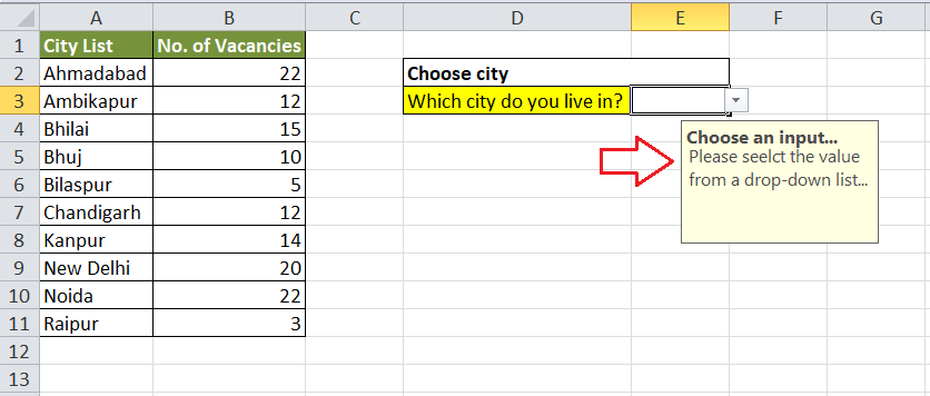
  Once we select the corresponding cell, our Input Message will look like this:
  
• If we want to display an error message to users giving wrong entries, we must go to the ‘Error Alert’ tab in the Data Validation window. There are different error alert types, such as an Information, Warning, and Stop. We can choose the desired error alert under ‘Style’ and enter the title and error message accordingly.
  
  If we now enter the data manually, we will see the customized error message with the error icon selected instead of the default message and icon.
  

Creating a Dynamic Drop-Down List

Unlike the static drop-down list, a dynamic drop-down list extends the possibility of adding or inserting new items based on the changes in the source range. This means if we want to add new items in our dynamically inserted drop-down list, we can simply add the individual item (s) in our source table.

For example, let’s retake the previous example sheet, where we have several names of the cities in cells from A2 to A11. If we insert two new cities in the cells below (A12 and A13), they will not automatically reflect in our static drop-down list inserted in cell E3.

However, when we have a dynamic drop-down list, the items get updated as soon as they are inserted in the source range or table.

Therefore, we need to create a dynamic drop-down list in a cell E3 by following the below steps:

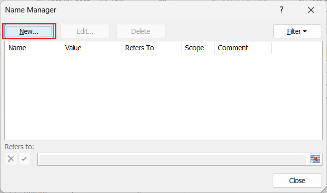
• First, we need to go to the Formulas tab and click on the ‘Name Manager‘ button.
  
• In the Name Manager tab, we must click on the ‘New‘ button.
  
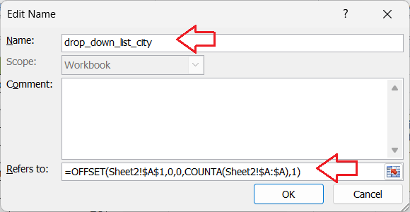
• In the next window, we need to give any desired name in the ‘Name‘ box and enter the OFFSET formula in the ‘Refers to‘ box, as shown in the following image:
  
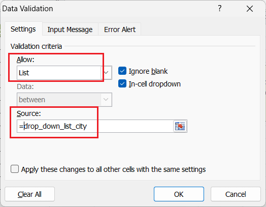
  After arranging the preferences in the ‘Name Manager’, we must click the OK button and the Close button.
• After that, we need to select the resultant cell E3 and go to Data Validation (Alt + A + V + V). Here, we must choose the ‘List’ option under ‘Allow’ and enter the created ‘Named Range’ in the ‘Name’ box. It will look like this:
  
  It is essential to ensure that the Named Range is entered correctly.
• Next, we can adjust the preferences in the following two tabs, Input Message and Error Alert. Once all the changes have been completed, we must click the OK We will see a dynamic drop-down list inserted in our cell E3, as shown below:
  
  After the dynamic drop-down is created, we can easily insert new items into the list. If we add a new city name to our table (cell A14), it is immediately reflected in our drop-down list.
  

Adding Items to created Drop-Down List

We can add new items in a created drop-down list, whether static or dynamic. However, there are some differences. In a static drop-down list, we can only insert a new item (s) by adding a new value(s) in the middle of the source range or table. If we add it at the end of the source range, it will not reflect in the drop-down list. However, a dynamic drop-down list gets updated based on given values in the source range, either in the middle or at the end.

For Static Drop-Down Lists

As stated before, we can only insert a new item somewhere in the middle of the source range when working with a static drop-down list. This is because the range selection in our drop-down list is limited by the first and last selected cells. However, when we insert an item in the middle of the range, Excel dynamically updates the range’s selection in the data validation rules. Further, it expands the range according to the number of cells we add in the middle of the source range.

We can perform the below steps to insert one or more new items in our static drop-down list:

• First, we need to press the right-click on any middle cell in our source range. In our example, the source range is A2:A11. So, we select cell A6 from the middle of the range and press the right-click here. Next, we must select the ‘Insert’ option from the list.
  
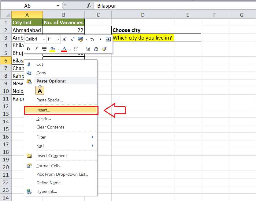
• In the next window, we need to select the radio button associated with the option ‘Shift cells down’ and click the OK button. We will see a new cell inserted in the middle of the range.
  
  Alternatively, we can also select the ‘Entire Row’ to insert based on the requirements of our data formatting. In our case, we insert the entire row.
  
• After that, we must type the desired item into an empty cell, which we want to insert into our static drop-down list. Lastly, we must press the Enter key.
  
  Now, if we check our drop-down list, we see a new item already inserted in a list that we just typed in an empty cell.
  

Note: To insert an item at the end of the static drop-down list, we must go to Data Validation settings and enter a new range in the Source box.

For Dynamic Drop-Down Lists

When dealing with the dynamic drop-down lists, we can follow the same procedure as discussed above for the static drop-down list and insert one or more new items in the middle of the list. Additionally, a dynamic drop-down list enables us to directly enter/ type an item at the end of the source range. As soon as we enter the item name at the end, it immediately reflects in the drop-down list.

Therefore, it is always recommended to use a dynamic drop-down list when there is a need for adding or inserting new item (s) in the future.

Deleting Items from created Drop-Down List

To delete any item from the drop-down list, we can simply delete the corresponding cell or row, and it works for both static and dynamic drop-down lists.

Dependent Drop-Down Lists

Sometimes, we may need to insert more than one drop-down list in our Excel sheet where one drop-down list depends on the selected entry on another one. We get different items in the second drop-down list based on the entry selected in the first drop-down list for each selected item in the first drop-down. It is called the dependent drop-down list or conditional drop-down list.

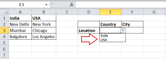
For example, suppose we have two drop-down lists in our sheet where the first drop-down contains the names of some countries while the second drop-down list displays the names of cities based on the country’s name selected in the first drop-down list.

If there is a chain of dependent drop-down lists controls, it is called cascading drop-down list. In that case, each drop-down list is dependent on the previous (or parent) drop-down list or selected entry.

We need to follow the below steps to create a dependent drop-down list in Excel:

• First, we need to select a cell (E3, in our case) to insert the first drop-down list. Next, we must navigate the Data tab > Data Validation > Data Validation. In a Data Validation window, we select the ‘List’ option and specify the ‘Source’ range (=$A$1:$B$1, in our case) that contains items to be displayed in the first drop-down list.
  
  Once all the preferences are set as above, we must click the OK button. This will immediately insert the first drop-down list.
  
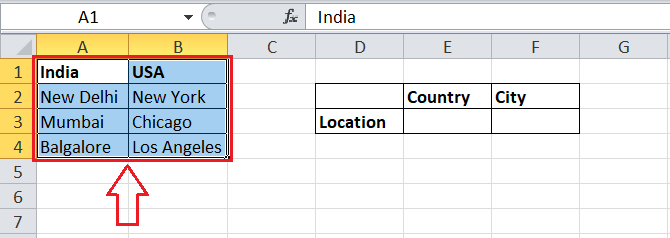
• After the first drop-down list is created, we must select the entire data set. In our case, we select the range A1:B4, as shown below:
  
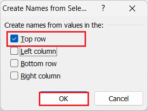
• Next, we must navigate the Formulas tab and click on the ‘Create from Selection’ button under the section ‘Defined Names’. This will launch another window.
  
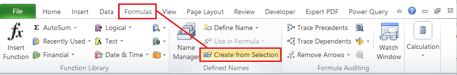
• We must only select/ tick the checkbox associated with the ‘Top row’ option in the next window and click the OK button. This will create two named ranges (‘Country’ and ‘City’), where the first name range (Country) will refer to the names of countries in the first list while another named range (City) will refer to the names of cities in the second list.
  
• After that, we need to select a cell to insert another (dependent) drop-down list. In our example, we select cell F3. Next, we navigate Data > Data Validation > Data Validation. In the Data Validation window, we again select the ‘List’ option and enter the formula =INDIRECT(E3) in the Source box. Here, the E3 represents the main/ parent drop-down list reference.
  
  It is essential to note that the INDIRECT function does not allow space characters in the named ranges. Besides, Excel automatically inserts an underscore for the spaces. So, if our main category has more than one word or space character (s), we must use the formula differently. For example, if we want to use any country name like ‘Sri Lanka’, we must use the formula =INDIRECT(SUBSTITUTE(E3,” “,”_”)) instead of traditional =INDIRECT(E3). The SUBSTITUTE function inside the INDIRECT function converts the spaces into underscores.
• Lastly, we must click the OK This will create a dependent drop-down list.
  
  In the above sheet, if we select different countries in the drop-down list 1, we see different city names in the drop-down list 2.
  

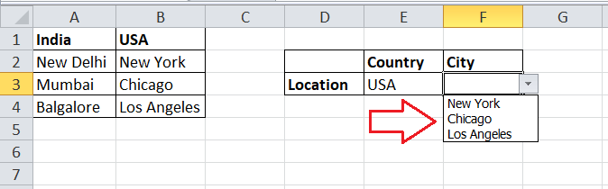
In this example, the conditional drop-down list (created in cell F3) refers to =INDIRECT(E3). When we select the ‘Country’ in cell E3, the drop-down list in cell F3 refers to the named range for the listed countries via the INDIRECT function. So, the corresponding function lists all the items (cities) in that specific category.

Important Points to Remember

• Excel also enables users to create a drop-down list using the custom items that are not even recorded in the sheet. In the Data Validation window, we can enter the items directly in the Source box by using Commas to separate them.
• We can copy drop-down lists from one cell to another using the shortcuts Ctrl + C (Copy) and Ctrl + V (Paste). However, if we don’t need the source formatting, we must use the Paste Special window (Ctrl + Alt + V) and select ‘Validation’ followed by the OK button.
• When working with the dependent drop-down lists, we must be more careful. If we make changes in the parent drop-down list, there will be no automatic changes in the dependent drop-down list. Therefore, we must double-check the dependent drop-down lists when edited.