Find and Replace in Excel

In Excel, if we want to search anything in our workbook like a specific number or text string, then we can use the Find and Replace features. We have the option of locating the search item for reference or replacing it with anything else. There are various wildcards that we can include in our search terms, such as asterisks, tides, question marks, and numbers. We can search by rows and columns, search within values or comments, and search with a worksheet or entire workbooks.

If we are working with a large amount of data in Excel, finding specific information can be challenging and time-consuming. We may use the Find feature to search our workbook, quickly and we can also use the Replace option to change the text.

When working with large Excel spreadsheets, it’s critical to be able to locate the information we need at any given time easily. Scanning hundreds of rows and columns is not the best way to proceed, so let’s take a deeper look at what Excel’s Find and Replace feature has to offer.

To Find Content

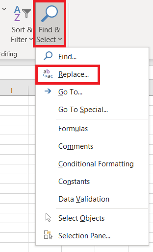
In order to find something in the workbook, we have to press Ctrl+F, or use another way that is we go to Home > Editing > Find & Select > Find.

Note: In this example, we will click on the options>> button in order to display the entire Find dialog. By default, it will display with options hidden.

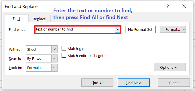
1. Firstly, in the Find what; box, we have to type the number or text which we need to find, or click the arrow in the Find what: box and then select a recent search item from the list.

Tips: In our search criteria, we can use wildcard characters such as an asterisk (*), question mark (?), and tilde (~).

• We can use asterisk (*) to find any number of characters. For example, s*d finds “sad” and “started”.
• We can use a question mark (?) to find any single character. For example, s?t finds “sat” and “set”.
• We can use tilde (~) followed by ?,*, or ~ in order to find question marks, asterisks, or other tilde characters. For example, fy91~? Finds “fy91?”.

2. Now, we have to click on Find All or Find Next to run our search.

Tip: When we click on Find All, a list of all occurrences of the criteria we are looking for appears, and clicking on a particular occurrence in the list will select its cell. By clicking a column heading, we can sort the results of a Find All search.

3. Next, we have to click on the Options>> in order to further define our search if required:

• Within: Select Sheet or Workbook to search for data in a worksheet or a whole workbook.
• Search: We have the option of searching By Rows (default) or By Columns.
• Look in: We have to click on the Formulas, Values, notes, or Comments in order to search for data with particular detail.

Note: Formulas, Values, Notes, and Comments are only available on the Find tab; only Formulas are available on the Replace tab.

• Match case: We can use this if we need to search for case-sensitive
• Match entire cell contents: We can use this option if we wish to search for cells that comprise only the characters, which we type in the Find what: box.
• If we wish to look for text or numbers with specified formatting, click Format and then use the Find Format dialogue box in order to make our choices.

Tip: If we wish to find cells that only match a particular format, then we can delete any criteria in the Find what box; after that, select a particular cell format. Choose Format From Cell by clicking the arrow next to Format, then clicking the cell with the formatting we wish to look for.

To Replace all Content

In order to replace text or number, we have to press Ctrl+H or go to Home > Editing > Find & Select > Replace.

Note: We’ve shown the whole Find dialog in the following example by clicking the Options >> button. It will open with Options hidden by default.

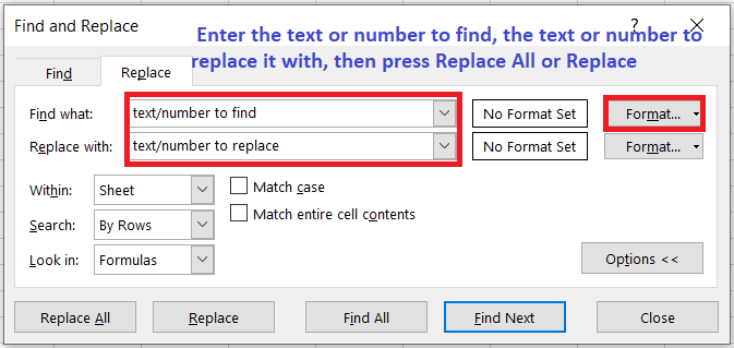
1. In the Find what: box, we have to enter the numbers or text that we need to Find, or we can click the arrow in the Find what: box and then select a recent search item from the list.

Tips: We can use wildcard characters such as asterisk (*), question mark (?), tilde (~) in our search criteria.

• We can use an asterisk (*) in order to find any number of characters, for example, s*t finds “sat and “subject”.
• We can use the question mark (?) in order to find any single character- for example, a?t finds “alt” and “apt” .
• We can use tilde (~) followed by ?,*, or ~ in order to find question marks, asterisks, or other tilde characters -for example, fy91~? finds “fy91?”.

2. Enter the text or numbers we need to replace the search text in the Replace with: box.

3. Click on the Replace All or Replace

Tip: When we click Replace All, it will Replace all occurrences of the criterion we’re looking for, whereas Replace will update one instance at a time.

4. Click Options> > in order to further define our search if necessary.

• Within: To search for data in a worksheet or in a whole workbook, select Sheet or
• Search: We have the option of searching By Rows (the default) or By Columns.
• Look in: To search for data with particular details, in the box, click Formulas, Notes, Comments or

Note: Formulas, Values, Notes, and Comments are only available on the Find tab; only Formulas are available on the Replace tab.

• Match case- If we want to look for case-sensitive, then we can use this.
• Match Entire Cell Contents: Select this option, if we wish to search for cells that only include the characters, we typed in the Find what: box.

5. If we wish to look for text or numbers with particular formatting, click Format and then use the Find Format dialogue box to make our choices.

Tip: If we need to find cells that only match a particular format, we can delete any criteria in the Find what box and then select a particular cell format as an example. Click the arrow next to the Format, click Choose Format From Cell, and then click on the cell, containing the formatting we need to search for.

Usage of FIND and REPLACE in Excel (Examples)

Excel’s Find and Replace feature can help us save a lot of time, which is what matters these days. In this tutorial, we will discuss some examples of usage of Find and Replace in Excel.

Example 1: To Find and Replace Formatting in Excel

This is a useful feature if we wish to replace old formatting with new formatting. For example, suppose we have cells with a yellow background color and wish to change the background color of all of them to orange. Rather than doing this manually, we can use Find and Replace to do it all at once.

The following are the steps to do this:

1. First, we have to select the cells for which we need to find and replace the formatting. If we need to find and replace a particular format in the whole worksheet, select the whole worksheet.
2. Go to Home -> Find and Select -> Replace (keyboard shortcut-control + H).
   
3. Next, we have to click on the options This will expand the dialogue box and display other options.
   
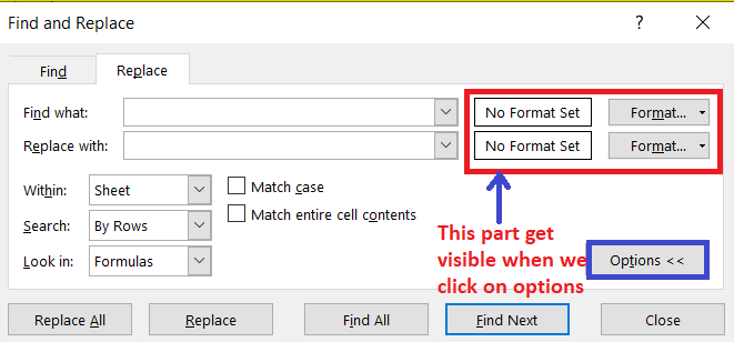
4. Click on the Find what Format button. A drop-down menu will appear, with two options: Format and Choose Format from cell.
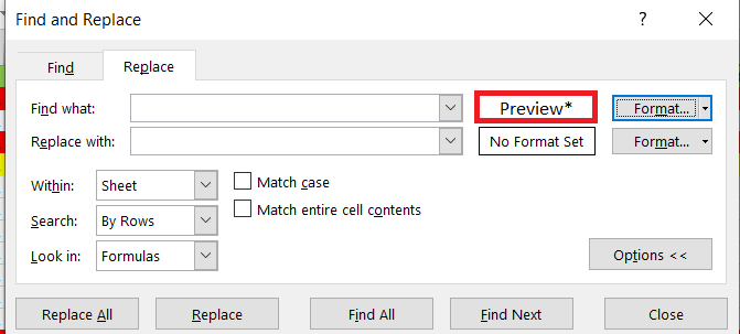
   • By clicking on the Format button, we can either manually specify the format we need to find or, select the format from the cell in the worksheet. In order to select the format from a cell, we have to select the ‘Choose Format from Cell’ option and then click on the cell from which we need to choose the format.
     
   • Once we select a format from a cell or specify it manually from the Format Cells dialog box, we will see it as a Preview to the left of the Format button.
     
5. Next, we have to specify the format which we want rather than the format we chose in the previous stage. Select Replace with Format button. It will display a drop-down menu with two options- Format and Choose Format from the cell.
   
   
   • We can specify it manually by clicking on the Format button or select an existing format from the worksheet by clicking on the cell that contains it.
   • We will get a Preview on the left of the format button whenever we select a format from a cell or manually define it from the format cells dialogue box.
     
6. Click on the Replace All

Example 2: To Add or Remove Line Break

What do we do when we have to move to a new line in an Excel cell?

We press Alt + Enter.

And what happens if we wish to revert this?

We delete it manually… right?

Assume we have a large number of line breaks which we need to delete. Manually deleting line breaks can take a long time, and we don’t have to accomplish this manually. Excel Find and Replace has a cool trick up its sleeve that will do this in a snap.

The following are the steps which we have to use in order to remove all the line breaks at once:

1. First, we have to select the data from which we need to remove the line breaks.
2. Go to Home -> Find and Select -> Replace (keyboard Shortcut-Control + H).
   
3. In the Find and Replace Dialogue Box:
   • Find What: Press Control + J (we may not see anything except a blinking dot.
   • Replace With: Space bar character (press space bar once).
     
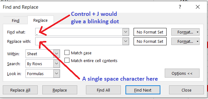
4. Click on Replace All.

Example 3: Find Cells with Formulas in Excel

As explained in Excel Find’s additional options, we can only search for a given value in formulas with Excel’s Find and Replace feature. Use the Go to special feature to find cells that comprise formulas.

Step 1: First, we have to select the range of cells in which we need to find the formulas or click any cell on the current sheet to search across the whole worksheet.

Step 2: Click on the arrow which is next to the Find & Select, and then we have to click Go To Special. Alternatively, we can enter F5 in order to open the Go To dialogue and click the special button in the lower-left corner.

Step 3: In the Go To Special dialog box, we have to select Formulas, then check the boxes next to the formula results we wish to find, then click Ok:

• Numbers: – Find formulas that return numeric values containing dates,
• Text: – Search for formulas that return text values.
• Logicals: – Find formulas that return Boolean values of TRUE and FALSE.
• Errors: – Find cells with formulas which result in errors like #N/A, #NAME? #REF!, #VALUE, #DIV/0!, #NULL!, and #NUM!

If Microsoft Excel finds any cells which satisfy our criteria, those cells will be highlighted; otherwise, a message will be shown that no such cells have been found.

Note: In order to quickly find all cells with formulas, regardless of the formula result, click Find and Select > Formulas.

Shortcuts for Find and Replace in Excel

The following are the shortcuts for Find and Replace in Excel:

• Ctrl+F: –In Excel, this shortcut is a Find shortcut that opens the Find tab of the Find & Replace.
• Ctrl+H: – In Excel, this shortcut is a Replace shortcut which opens the Replace tab of the Find & Replace.
• Ctrl+Shift+F4: – This shortcut is used to identify the prior occurrence of the search value.
• Shift+F4: – This shortcut is used to Find the next occurrence of the search value.
• Ctrl+J: – We used this shortcut to find or replace a line break.