Filters in Excel
Example – easy filtering by category in Excel
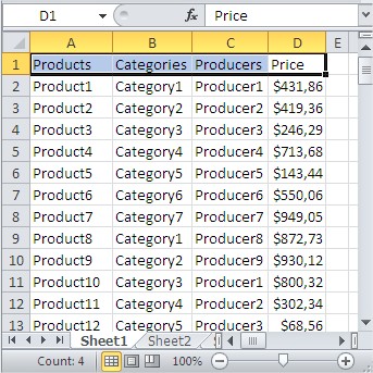
You will use a table of products which filters them by category.

Select the table header row.

Go to the Ribbon. In the Home tab, click the Sort & Filter icon and select Filter from the list.

In the table appeared some buttons to filter the data.

Click on the Categories. In the list untick the category which you want to be hidden (filtered), such as Category2.

After applying a filter, you can’t see products from Category2.

On the picture above you can also see that some rows are hidden. You don’t see 3 and 10 row. In the B1 cell you can also see a symbol of filter close to the arrow. That means that this column is filtered.
If you want to filter more you can. Let’s hide products from Producer3 and Producer5.

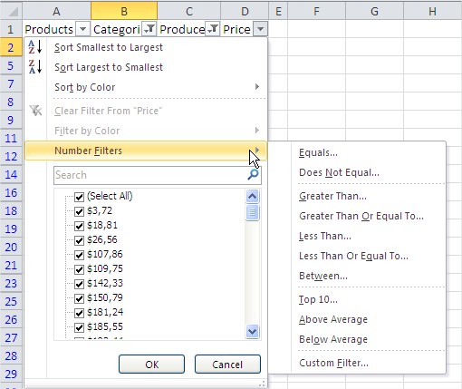
You can also filter prices. There’s more number filters. Click filter arrow in D1 cell.

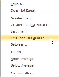
I want to find the cheapest. I select Less Than Or Equal To.

My budget is $150.

That’s how I filtered out products which I don’t want in my table.

Now it is much easier to choose one.


