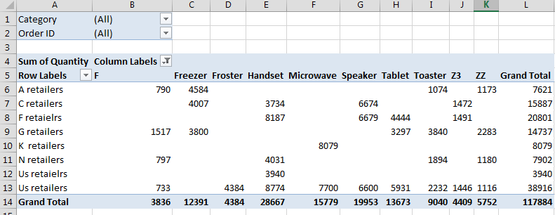
Filtering Top 10 Pivot Table Values
 2. Now select the head you want to filter.
3. Now, go to value filter and select top 10. A dialog will appear. (Set the criteria the way you like).

4. Finally, click ok. Your pivot table is filtered.

Template
You can download the Template here – Download
Further reading:
Basic concepts
Getting started with Excel
Cell References


