Excel sumif Function

The SUMIF function is used to sum up the values of some specific cells of a column, the cells which meet certain criteria. SUMIF is a conditional function used to sum the value of any particular cell in a column. SUMIF function is one of the eight functions of a function group in Excel.

Sometimes, a user requires to total the values that satisfy to the criteria set by the user. You can easily do it using the SUMIF method. SUMIF function helps the users to sum up column data along with a condition. We will brief you SUMIF function to sum a column values based on a condition.

Essential Points

1. SUMIF function supports only one condition. So, do not use this function for multiple conditions.
2. Excel provides the SUMIFS function for multiple criteria.
3. Enclose the text string condition in double quotes (“”).
4. Wildcard characters, such as ? and * can be used in the SUMIF function.

Syntax

Arguments

The SUMIF function has three main parameters, which are permanent:

Range: It refers to the range of cells that you want to evaluate to shortlist the cells that meet the given criteria.

Criteria: It refers to conditions that tell which cells are to be added. It can be a number or a text.

Sum _range: It provides the actual cells that are to be added. It is an optional argument. If we omit this part of the function the SUMIF function treats “range” as “sum_range” thus adds the cells of the range argument.

Return Value

The SUMIF function returns the sum of the cells of a column that meets or satisfies the specified condition.

How SUMIF is different from Subtotal

SUMIF function is a function used in an Excel spreadsheet to total a column value with some condition. This function helps to total the column data only, which satisfies the defined criteria.

Although, SUMIF is a bit similar to the Subtotal method because both SUMIF and Subtotal method does not total the entire column data. The Subtotal method is used after applying the filter to the column, whereas SUMIF can be used directly on a table with the condition.

In simple terms, you can say that the SUMIF function executes on a normal Excel spreadsheet while the Subtotal function only applies to filtered table data to total a column data.

Now, let’s see how the SUMIF function is used to calculate the sum of column data with some conditions on it. Let’s understand with an example –

Sum a column values based on criteria using SUMIF

Example 1: SUMIF

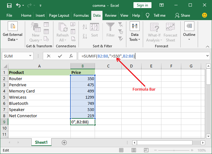
We have a dataset of products and their price. We will calculate the sum of all products whose price is greater than 550. Remember that the table data is not filtered. So, do not confuse.

Use the following SUMIF formula and get the total of the cells which satisfy the defined condition.

Follow the steps to calculate sum using the SUMIF function:

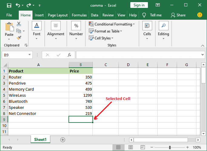
Step 1: Open your worksheet, select the cell where you want to paste the result.

Step 2: Go to the Formula bar and paste the above formula in it.

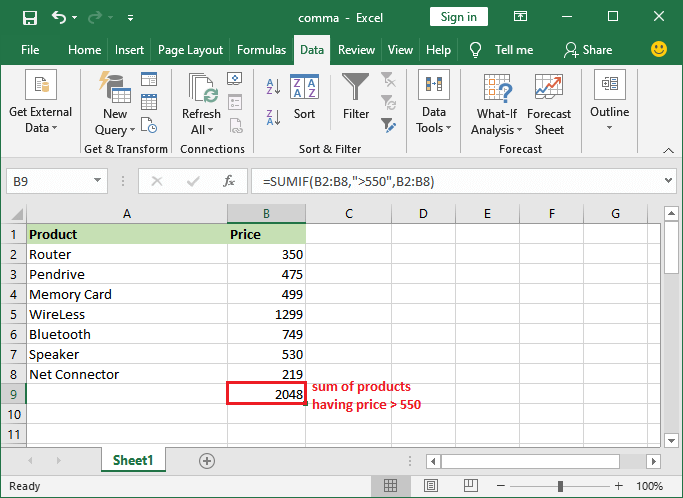
Step 3: Press the Enter key to get the result.

Note: You can use the SUMIF formula on numeric as well as test conditions.

Suppose we have to calculate the total sum of all pen drives present in this spreadsheet. In that case, use Pen drive as the condition and include both A and B columns, i.e., Product and Price.

Example 2: SUMIF

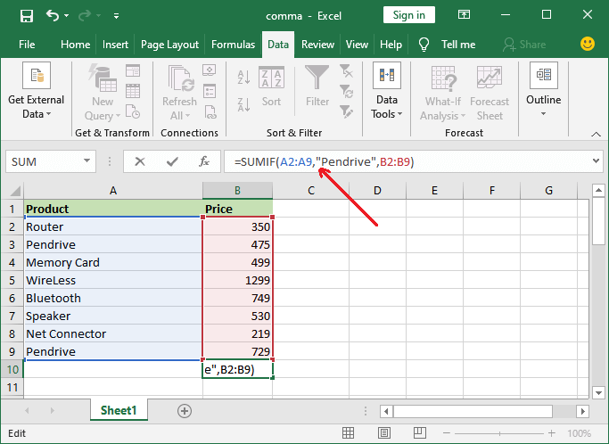
In this example, we will use the same Excel table data as used in the above example containing a dataset of products and their price. We will calculate the sum of all pen drives present in this Excel list. It requires a bit different formula than the above example.

Use the following SUMIF formula and get the total of the cells which satisfy the defined condition.

Step 1: Open your worksheet, select the cell where you want to paste the result.

Step 2: Copy and paste the following SUMIF formula in the formula bar:

Step 3: Press the Enter key and get the total prices of pen drives present in this Excel spreadsheet.

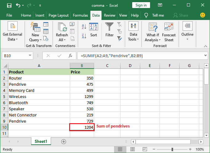
Here, you can see that we have two Pen drive products of different prices in this table. This time you will see that the sum is calculated of two pen drives whose total price is 1204 as calculated in the above step.

Some Important formulas

You can also use the SUMIF function as shown below:

Besides that, SUMIFS is another function that is almost similar to the SUMIF.