Excel Rank Function
You are given a list of sales data of different sales candidates, and you are asked to find out their Rank from largest to smallest to conclude who performed the best. Now you might think of applying various formulas to solve the above problem or even manually doing it. But why go the hard way when Excel has already provided an inbuilt function named “RANK” that will help you to rank numeric data values from largest to smallest and vice versa.
What is RANK function?
The Excel RANK is an inbuilt function used to return the rank of a specific number for a given list of numeric data values. In simple words, this function returns the statistical rank of a specified value within a provided array of values. The RANK function is capable of ranking the data values from smallest to largest and largest to smallest.
The RANK function comes under the category of Excel Statistical functions. It is not required to sort the data values in ascending or descending order before applying RANK.
Although this function has been replaced with advanced Excel functions, it is advisable to start using the new functions that may give you improved accuracy. When you type RANK in Excel, you will see the following suggestions:

In the above image, you will notice the RANK function; there is a yellow triangle with an exclamation mark. It represents that this function is may not be available in future versions, so it’s better to get used to RANK.AVG and RANK.EQ functions.
Note: The RANK formula is a predefined set-up for a formula capable of extracting and displaying values using a sort order in an Excel helper column.
Syntax
Parameters
- Number (required): This parameter represents the number whose rank you wish to find in your Excel worksheet.
- Ref (required): This parameter represents an array of, or a reference to, a list of numbers. Always remember that the nonnumeric values in ref are ignored.
- Order (optional): This parameter represents a number that specifies in which order you wish to rank the number in Excel.
- If the argument order is 0 (zero) or omitted, Excel ranks the given number as if ref were a list sorted in descending (largest to smallest) order.
- If the argument order is any value other than zero, Excel ranks the given number as if ref were a list sorted in ascending (smallest to largest) order.
Points to Remember:
- The default value for the ‘order’ argument is zero (0). If the argument order is 0 (zero) or omitted, Excel ranks the given number as if ref were a list sorted in descending (largest to smallest) order. The highest number will be ranked #1, the second higher will be ranked as 2 and so on. The smaller the number the higher will be the rank.
- If the order value is 1, the numbers will be ranked against the numbers sorted in ascending order. The smallest number will be ranked #1, the second smallest will be ranked as 2 and so on. The highest the number the higher will be its rank.
- It is not mandatory to sort the values in the list before using the RANK function.
- If you have exact same value in the specified range, in that case the RANK() function will allot the same rank value to each value.
- Some documentation may claim that the parameter ‘ref’ can be a range or array, but it the parameter ‘ref’ must be a range.
Example 1: Using the Excel RANK formula find the RANK of achieved sales target for employee named Elena Gilbert. The table is given below.
| Name of Employee | Sales Target achieved |
|---|---|
| John Sudds | $5,600 |
| Eric | $4,367 |
| Abdullah Madina | $6,578 |
| Itrat Zaidi | $3,456 |
| Rajat Garg | $3,456 |
| Elizabeth | $3,234 |
| Elena Gilbert | $5,643 |
| Steward Forbes | $5,345 |
To find out the rank of an employee follow the below given steps:
STEP 1: Add a helper column named Rank
Put your mouse cursor to the cell next to “Sales target achieved” and Type Rank on top of it.
It will look similar to the below image:
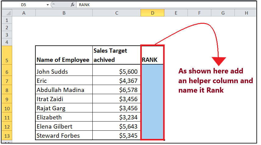
In this column we will enter the formula and will find out the RANK of various numeric data values.
NOTE: You can also format this column unlike others to make your Excel worksheet more visually appealing.
STEP 2: Insert the formula
Move to the second row and start typing the formula = RANK(
It will look similar to the below image:

STEP 3: Add the parameters
- The first parameter represents the input value of the rank you want to calculate. Here, C6 represents John’s sales target, i.e., $5600.
It will look similar to the below image:
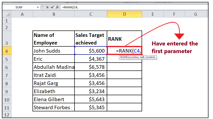
- In the 2nd parameter, you are required to specify the total cells containing the sales target are from C4 to C11. So, the range is C4:C11, which includes the sales target achieved by all the employees in a month.
It will look similar to the below image:
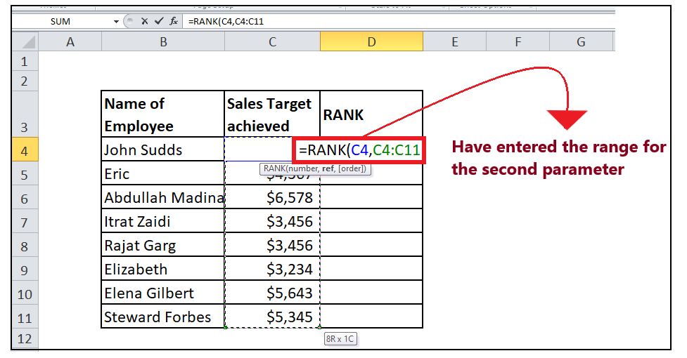
- In the third parameter, you will be requested to specify the order. As we want to rank it in the descending order (largest to smallest), we will pass 0 as value. If you want you can skip this parameter as its optional and default value is 0.
It will look similar to the below image:

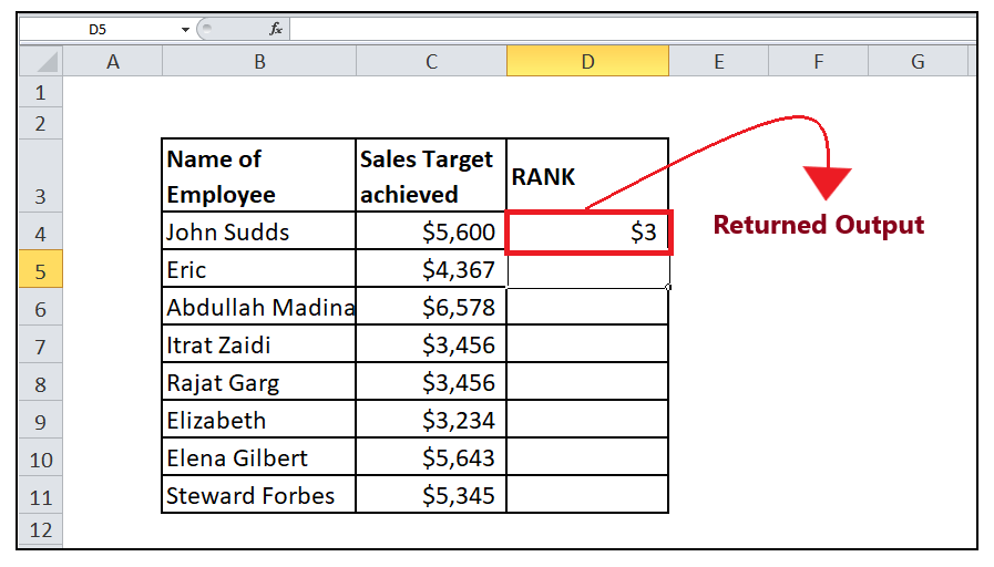
STEP 5: Rank will return the result
RANK (C4, B4: C11, 0) will return the rank of the employee named John Sudds as $3.
STEP 4: Drag the formula to other rows to repeat
Put your cursor on the formula cell and take it towards the right of the rectangular box. You will notice that the cursor will change into ‘+’ icon.
It will look similar to the below image:
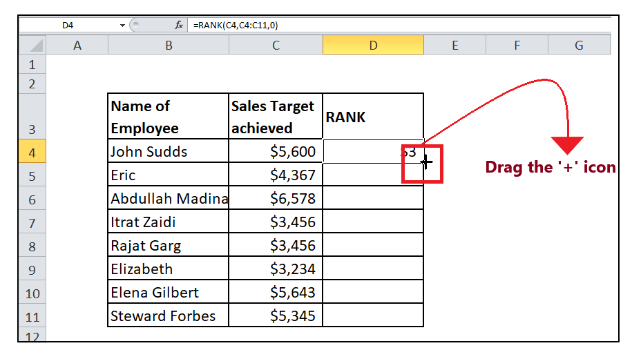
Drag the + icons to all the cells below it. This will automatically copy the RANK function to all the cells.
Refer to the below image:

STEP 5: Look for Elena Gilbert’s Ranking
As now all the ranks are out. Look for Elena Gilbert and check what her rank is. Here, in cell D10 it is denoting that Elena Gilbert has secured 2nd rank.
It will look similar to the below image:

By default, RANK will assign 1 to the highest value found in the data array, 2 to the second highest data, and like this it will keep the ranking on. This procedure works flawlessly unless and until all the array values are unique. However, if it finds two same numeric values it gives them the same ranking. Unlike, in the above image you can see cell D7 and D8 have same ranking because both have identical numeric values.
Example 2 – Calculate John’s Rank in Computer
| Student ID | Marks Obtained |
|---|---|
| John | 90 |
| Steve | 70 |
| Rahul | 20 |
| Paul | 41 |
In the above example, the Marks of the Students in computer and English subjects are shown. To find john’s rank in computer, we would use the Excel RANK function and follow the below given steps:
STEP 1: Add a helper column named Rank
Put your mouse cursor to the cell next to “Marks obtained” and Type Rank on top of it.
It will look similar to the below image:

In this column we will enter the formula and will find out the RANK of various numeric data values.
NOTE: You can also format this column unlike others to make your Excel worksheet more visually appealing.
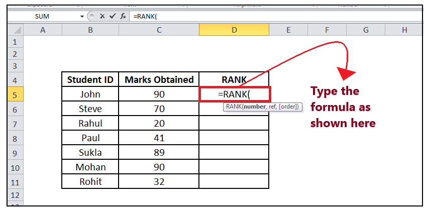
STEP 2: Insert the formula
Move to the second row and start typing the formula = RANK(
It will look similar to the below image:
STEP 3: Add the parameters
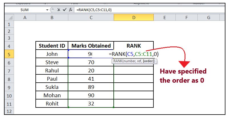
The first parameter is the input value, of which the rank is to be calculated. Here, B6 represents Steve’s marks in computer, i.e., 70.
It will look similar to the below image:

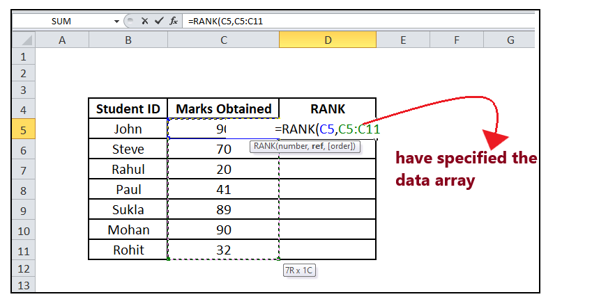
The 2nd parameter, the total cells containing computer marks are from C5 to C11. So, the range is C5:C11, which comprises all students’ marks in computer.
It will look similar to the below image:
In the third parameter, you will be requested to specify the order. As we want to rank it in the descending order (largest to smallest), we will pass 0 as value. If you want you can skip this parameter as its optional and default value is 0.
It will look similar to the below image:
STEP 5: Rank will return the result
RANK (C4, B4: C11, 0) will return the rank of the employee named John as $3.
STEP 6: Drag the formula to other rows to repeat
Put your cursor on the formula cell and take it towards the right of the rectangular box. You will notice that the cursor will change into ‘+’ icon.
It will look similar to the below image:
Example 3: Use the RANK formula to rank race results
| Student ID | Race Results |
|---|---|
| John | A1 |
| Steve | C2 |
| Rahul | F |
| Paul | A2 |
| Sukla | B1 |
| Mohan | B2 |
| Rohit | C1 |
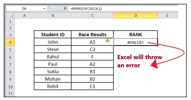
In the above table, instead of the numeric range, we have text. Let’s see what happens when we apply the RANK formula for text values.
To find out the rank of race results follow the below given steps:
STEP 1: Add a helper column named Rank
Put your mouse cursor to the cell next to “Race Results” and Type Rank on top of it.
It will look similar to the below image:

In this column we will enter the formula and will find out the RANK of various numeric data values.
STEP 2: Insert the formula
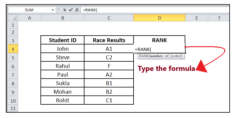
Move to the second row and start typing the formula = RANK(
It will look similar to the below image:
STEP 3: Add the parameters
- The first parameter represents the input value of the rank you want to calculate.
- In the 2nd parameter, you are required to specify the total cells containing the array of cells.
- In the third parameter, you will be requested to specify the order. As we want to rank it in the descending order (largest to smallest), we will pass 0 as value. If you want you can skip this parameter as its optional and default value is 0.
It will look similar to the below image:

STEP 4: Excel will throw #value! Error
This function is made specifically to rank numeric data values, but here we have entered non numeric data. Therefore it will throw #Value! Error stating that the values used in the function are of wrong data type.
