Excel ODD Function
When you hear the name of ODD for the first time, it may sound like some normal function that tells whether a number is odd or not. But that definition is not limited to this as you can integrate the Excel ODD function with other functions and solve various complicated problems.
In this tutorial, we will discover the basic and advanced applications of the Excel ODD function using several examples such as its usage will become crystal clear.
What is Excel ODD Function?
The Excel ODD function rounds a positive number up and negative number down to the nearest ODD integer. For example if you pass the following input =ODD (-2.5), this function will return the rounded output of -3, and if the specified input is =ODD(2.5) then the returned output will be 3.
The Excel ODD function returns a numeric value by rounding the specified number to the next odd integer. ODD function always rounds numbers away from zero. Therefore, the positive numbers become larger and negative numbers become smaller (i.e., more negative). This function takes just one parameter (number), which should be a numeric value. If you pass non-numeric in its argument, it will throw a #VALUE! error.
Syntax
Parameters
Number (required): This parameter represents the cell which you want to convert to the nearest ODD integer.
Return
This function returns an ODD integer after rounding a positive number up and negative number down to the nearest ODD integer.
Points to Remember about ODD Function
- The ODD function only works with numeric values.
- The ODD function returns the nearest next odd integer for any specified decimal number.
- The function returns the number away from zero.
- The ODD function only works for numeric values. If you supply any non-numeric value in its parameter, it will throw #VALUE! error.
- If you pass zero (0) and numbers that are already odd integers in its argument, no rounding occurs.
Example
Example 1: Use ODD function to round off the number on the following examples.
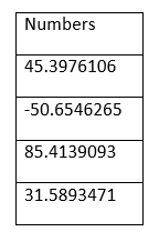
Follow the below steps to round off the numbers to its nearest ODD number:
STEP 1: Insert a helper column
Add a column next to “Numbers” and type the column name “ODD Round off” on top of the cell.
It will look similar to the below image:
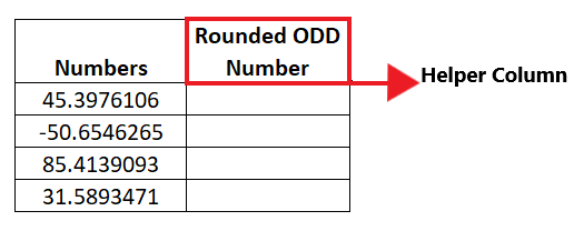
In the helper column, we will type the ODD function for every row and find round off the numbers to its nearest ODD number.
NOTE: As the above image shows, we have formatted the column with borders and font to make the worksheet more visually attractive.
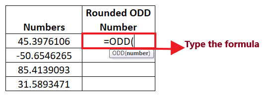
STEP 2: Insert the ODD formula
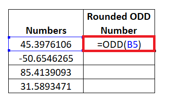
The next step is to enter the formula so put your cursor in the second row of your helper column start typing: = ODD(
It will look similar to the below image:
STEP 3: Add the number parameter
The first parameter includes “Number” which represents the cell which you want to convert to the nearest ODD integer. Here, cell reference B4 holds our numeric value. So our formula becomes: =ODD (B5)
It will look similar to the below image:
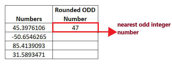
STEP 4: ODD will return the nearest ODD integer number
ODD (B5) will return the ODD integer number after rounding it off to its nearest ODD number.
STEP 5: Drag the formula to other rows to repeat
Put your cursor on the formula cell and take it towards the right of the rectangular box. You will notice that the cursor will change into the ‘+’ icon.
It will look similar to the below image:

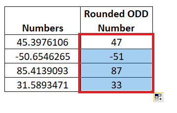
Drag the + icons to all the cells below it. This will automatically copy the ODD function to all the cells. As a result, ODD will return the integer numbers after rounding it off to its nearest ODD number.
STEP 6: Explanation of each Output
- The first number in the above table was 45.3976106. When we applied the ODD function for this number, it returned its nearest ODD integer value, i.e., 46. This function rounds the given numeric values away from zero, so the positive values become larger, and therefore it returned 47.
- For the second number, a rounded negative odd number for -50.6546265 is 52. This function rounds the given numeric values away from zero numbers away from zero, so the negative numbers become smaller, and therefore it returned -51.
- For the third number, the rounded odd number for 85.4139093 is 87.
- The same applies for the fourth value, and the odd rounded number for 31.5893471 is 33.
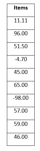
Example 2: In the below table, find all the odd numbers using the Excel ODD Function and count how many ODD numbers are there in the list.
To find the count of odd numbers from the above list, we will use a combination of Excel ODD and COUNTIF function. Follow the below given steps to achieve the same:
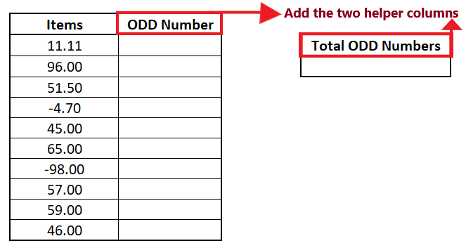
STEP 1: Insert two helper columns
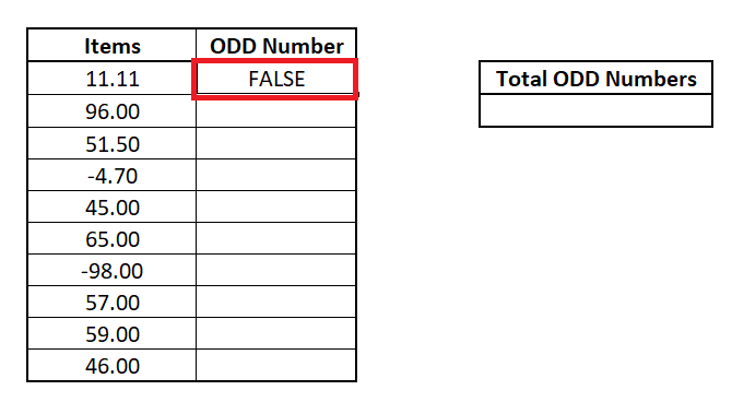
- Add a column next to “Numbers” and type the column name “ODD Number” on top of the cell.
- Add another helper column and name it “Total Odd number.”
It will look similar to the below image:
- In the first helper column, we will apply the ODD function and check for each given number, whether is it is EVEN or ODD.
- In the second helper column, we will apply the COUNTIF function and count the odd numbers present in our list.
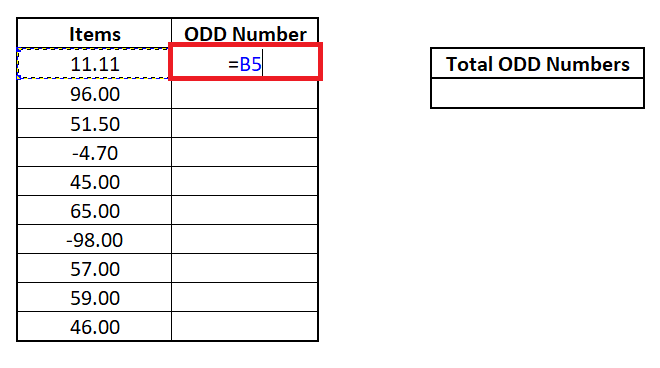
STEP 2: Insert the formula = cell reference
The next step is to enter the formula. Start the formula with the = (sign), and then we will pass the reference of our data cell. In our case, our data is in cell B5, so our formula becomes: =B5
It will look similar to the below image:
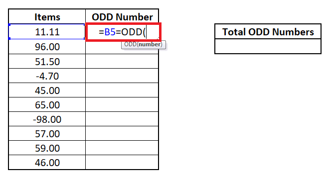
STEP 3: Insert the ODD formula
- We will compare the above formula with the output of the ODD function. Type the ‘=’ sign and enter the formula by typing: = B5 = ODD(
It will look similar to the below image:
- Include the first parameter “Number” which represents the cell which you want to convert to the nearest odd integer. Here, cell reference B4 holds our numeric value. So our formula becomes: = B5 = ODD(B5)
It will look similar to the below image:
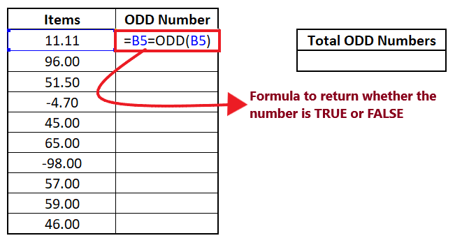
The above formula will check whether the value in cell B5 is equal to the closest ODD number. If it is equal, it will return TRUE; if it is not equal, it will return FALSE.
STEP 4: Formula Will return Boolean False
The combination of above formula will return a Boolean value False since A2 (11.11) and ODD (11.11) are not equal.
STEP 5: Drag the formula to other rows to repeat
- Put your cursor on the formula cell and take it towards the right of the rectangular box. You will notice that the cursor will change into the ‘+’ icon.
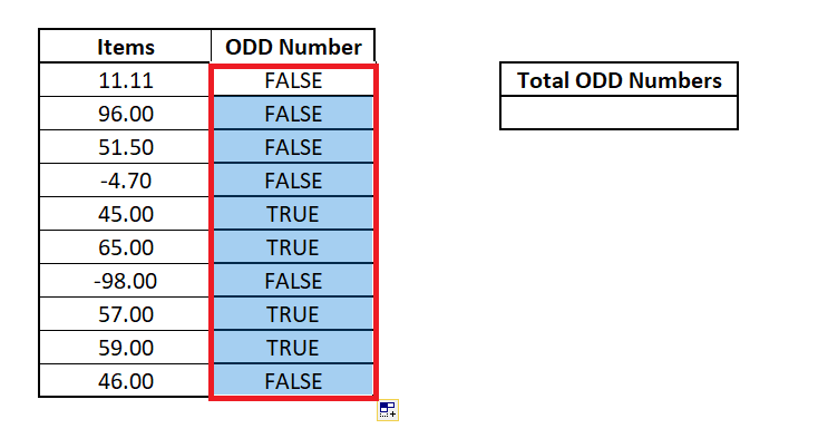
- Drag the + icons to all the cells below it. This will automatically copy the ODD function to all the cells. As a result, ODD will return the integer numbers after rounding it off to its nearest odd number.
You will have the following Boolean outputs:
STEP 6: Apply COUNTIF formula to get the total count of even numbers
We will use the Excel COUNTIF formula in cell E6 to get the total count of all TRUE values, in the list. So the formula will be as follows:
Refer to the below image:
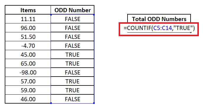
STEP 7: COUNTIF will return the total number of even numbers
Here COUNTIF formula will count all the TRUE values present in the range C5: C14 and return the sum of all the TRUE values. The total number of TRUE values in the range C5: C14 is 4. That means there are 4 odd numbers in the list.

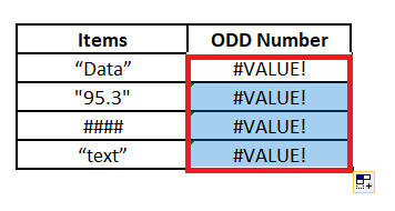
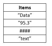
Example 3: In the below table we have some data inputs that are non-numeric, let’s see what happens when we use the Excel ODD Function.
Follow the below given steps to achieve the same:
STEP 1: Insert a helper column
Add a column next to “Items” and type the column name “ODD Number” on top of the cell.
It will look similar to the below image:
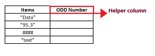
In the helper column, we will check for each given number whether is it is EVEN or ODD.
STEP 2: Insert the ODD formula
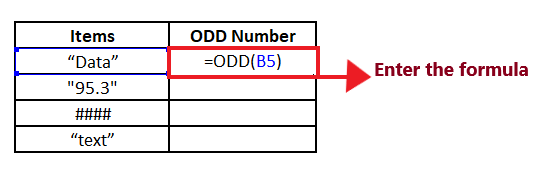
- Enter the formula so put your cursor in the second row of your helper column start typing: = ODD(
- Include the parameter “Number” which represents the cell which you want to convert to the nearest even integer. Here, cell reference B4 holds our value. So our formula becomes: = ODD(B5)
It will look similar to the below image:
STEP 3: ODD will return an error
The ODD function only works for numeric values. If you supply any non-numeric value in its parameter, it will throw an #VALUE! error. In the B5 cell, we have supplied string values. Therefore the ODD (B5) formula has returned the #VALUE! error as shown in the below image:
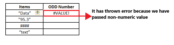
When you drag the formula for the rest of the cells, you will find the same #VALUE! error because all the values are non-numeric.