
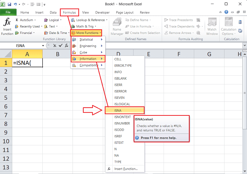
Excel ISNA Function
MS Excel is powerful spreadsheet software that allows users to record large amounts of data and perform various operations using many built-in functions. While using functions and formulas within an Excel sheet, various scenarios can make us face some error codes instead of the desired results. However, it would be difficult to identify or detect such errors directly with our eyes when working with large data sets. This is where an existing function ISNA comes in handy and helps us identify or detect a specific type of error in our worksheets.
This article discusses the brief introduction of the Excel ISNA function along with its syntax, purpose, and procedure to use in our Excel worksheets. We discuss some relevant examples to help us better understand how to use the ISNA function in Excel for various common scenarios.
What is ISNA Function in Excel?
The ISNA function is one inbuilt error-handling Excel function categorized under the Information Functions. The function is particularly helpful in finding or handling only the #N/A errors with the worksheet. In simple words, the ISNA function in Excel helps us identify whether the given set of data, function, or formula has the #N/A error or not. The function makes it easier to facilitate smooth comparisons and data analysis and helps fix the errors accordingly.
Additionally, the ISNA function can be combined with other relevant functions like the IF or VLOOKUP functions to perform additional operations on the recorded data sets within the worksheet.
Syntax of Excel ISNA Function
The syntax of the ISNA Function in Excel is defined as below:
The ‘value’ is the only desired argument or parameter by the ISNA function.
Arguments/ Parameters of Excel ISNA Function
As illustrated in the preceding syntax, the ISNA function in Excel only requires a single parameter, such as:
- Value: It is a flexible, mandatory parameter and represents the data to be tested for the #N/A error. It can denote another function, formula, cell, range, or direct value. Generally, the ‘value’ is given in the form of a cell address/ reference or a range.
What does the Excel ISNA function return?
The ISNA function in Excel returns a logical value, either TRUE or FALSE:
- TRUE: The function returns TRUE only if a #N/A error exists for the given ‘value’ parameter.
- FALSE: The function returns FALSE if no #N/A error is found for the given ‘value’ parameter. In that case, the given parameter may contain other values or error types.
For instance, take a look at the following table that determines how the ISNA Excel function behaves for the different data sets (parameters):
| Data | Formula | Returns | Description |
|---|---|---|---|
| #N/A | =ISNA(#N/A) | TRUE | Since the given value is the #N/A error, the ISNA function returns TRUE. |
| #DIV/0! | =ISNA(#DIV/0!) | FALSE | Although the supplied value is an Excel error, it is not the #N/A error. So, the ISNA function returns FALSE. |
| #NAME? | =ISNA(#NAME?) | FALSE | Since the given value is not the #N/A error, the ISNA function returns FALSE. |
| Text | =ISNA(Text) | FALSE | The ISNA function does not recognize text values as valid arguments and returns FALSE. |
How to use the ISNA Function in Excel?
It is better to use the ISNA function in an excel worksheet by using a sample data set to understand this function’s concept completely. Let us consider the following examples and use the ISNA Excel function in different cases:
Example 1: General ISNA Function
As in the table above, we used the ISNA function in its pure form. However, the ISNA function is more often used by combining it with other essential functions that help evaluate the results of the corresponding formula in our sheet. In such cases, we usually apply the ISNA function in the following way:
=ISNA(another_formula() )
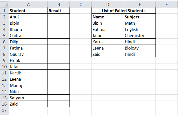
Suppose we have an example dataset with two lists of students’ names in columns A and D. The list in column A contains all students’ names, while column D only contains those who have failed exams.
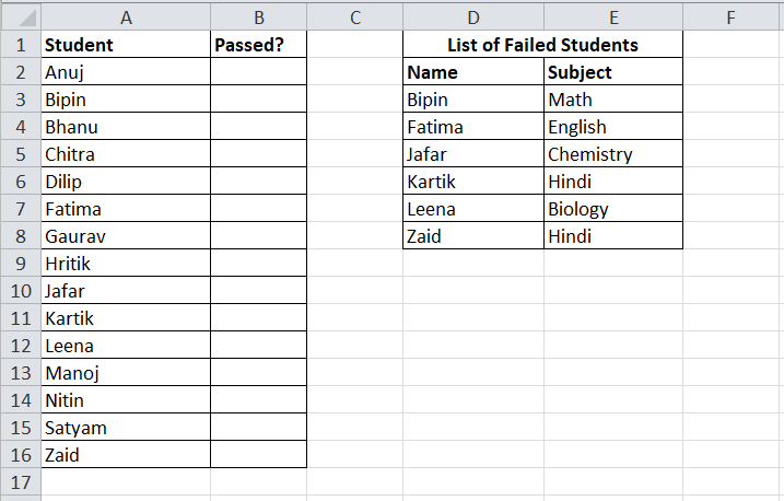
We need to compare both lists and identify whether the specific name is present only in the first list or in both lists. Later, we need to use the ISNA function to know whether the student in column A has passed or failed.
To compare the names of the first student (cell A2) against each respective name in column D, we can apply the MATCH formula in the following way:
=MATCH(A2, $D$3:$D$8, 0)
This formula will match the value of cell A2 into column D (from cell D3 to D8) and return its relative position if the value is present. The formula will return the #N/A error if the value does not match. So, we can combine or nest the above formula within the ISNA function that will return TRUE, where the MATCH function against the students’ names gives the #N/A error, meaning the corresponding name is not present in the list of failed students.
We can nest the MATCH formula within the ISNA function in the following way:
=ISNA(MATCH(A2, $D$3:$D$8, 0))
We apply this formula in cell B2 and copy it down to other cells till B16.

The image shows that the ISNA function has returned Boolean values TRUE and FALSE. We can see here that the function returns TRUE for students who are not listed in column B. Let’s understand the working of the ISNA function when it returns TRUE and FALSE:
- TRUE: a student name is not found in column D > MATCH function returns #N/A error > ISNA returns TRUE.
- FALSE: a student name is found in column D > MATCH function returns no error > ISNA returns FALSE.
Example 2: ISNA Function with the IF Function
As we said above, the Excel ISNA function only returns the Boolean value TRUE and FALSE. However, we can combine the ISNA function with the IF function to return or display a custom message. This makes the use of the ISNA function more effective to some extent. In such cases, we usually apply the ISNA function in the following way:
=IF(ISNA(…),”message_if_error_exists”, “message_if_no_error_exist”)
Let us again take the previous example data set. However, instead of showing Boolean TRUE and FALSE results, we need to display a custom message this time. Suppose we want to display a message ‘Passed’ for students who have not failed (who have not their names listed in column D). We want to display the message ‘Failed’ for the remaining students.
First, we apply the MATCH function, and later we nest it inside the ISNA function just like the previous example. After that, we embed the ISNA MATCH formula within the IF function in the following way:
=IF(ISNA(MATCH(A2, $D$3:$D$8, 0)), “Passed”, “Failed”)
Like the previous example, we apply the formula in cell B2 and copy or drag it to other remaining cells in the column through B16.

Compared to the previous example, the results look much better and more intuitive this time.
Example 3: ISNA Function with the VLOOKUP Function
The VLOOKUP function in Excel is one of the most widely used built-in functions that help us extract data from one list to another sheet. However, getting a #N/A error in the VLOOKUP formula is very common. The error usually occurs when the function does not find the lookup value in the given data set.
Instead of displaying the #N/A error in the resultant cell, displaying some meaningful message or a blank space is better. This will make our visual representation effective and more professional. The ISNA function comes in handy in such situations. After the ISNA function is combined with the VLOOKUP function, it helps determine whether the #N/A error exists in the given data set. Later, we can nest the combined formula of ISNA and VLOOKUP functions within the IF function to return or retrieve a customized message in place of the #N/A error.
The syntax of the ISNA function with the VLOOKUP can be defined as below:
=IF(ISNA(VLOOKUP(…),”custom_message”, VLOOKUP(…))
This formula returns the ‘custom message’ when there is a #N/A error in the given dataset; otherwise, it returns the result obtained by the VLOOKUP function.
In our example data set, suppose we want to display the subject’s name for those who have failed. We need to display a custom message ‘All Passed’ for others who have passed the exams.

First, we need to construct the classic VLOOKUP formula following the syntax below:
=VLOOKUP (lookup_value, table_array, col_index_num, [range_lookup])
- lookup_value: a value that we need to look up, i.e., students’ names or the corresponding cell references.
- table_array: a range that consists of the lookup value, i.e., D3:E8. We use absolute reference ($D$3:$E$8), so the references do not change when copied to other cells.
- col_index_num: a column number from the given table_array (or range) from where the matching value must be retrieved.
- range_lookup: the way we want to look up. We must use TRUE (or 1) for an approximate match and FALSE (or 0) for an exact match.
So, we look up the desired subject using the below VLOOKUP formula:
=VLOOKUP(A2, $D$3:$E$8, 2, FALSE)
After that, we have to combine this VLOOKUP formula with the generic IF-ISNA formula discussed in the previous example. Thus, our entire formula becomes this:
=IF(ISNA(VLOOKUP(A2, $D$3:$E$8, 2, FALSE)), “All Passed”, VLOOKUP(A2, $D$3:$E$8, 2, FALSE))
We apply this formula in our first resultant cell, B2, and copy it down to the remaining cells till B16.
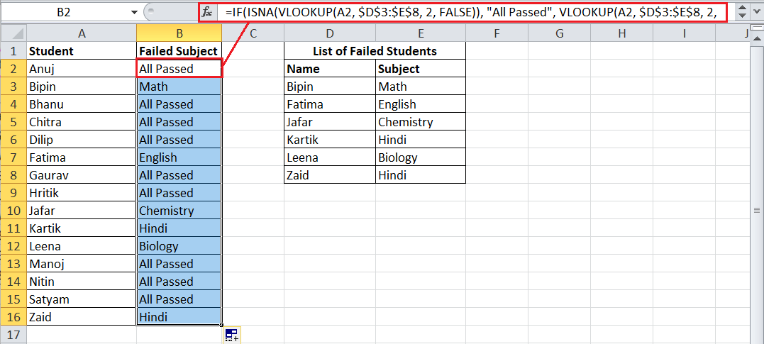
The above image shows the subject names of the students who have failed. For remaining, we see a custom message ‘All Passed’. Now replace the ‘All Passed’ custom message with a dash (-). It highlights our desired results more effectively, as shown below:

Example 4: ISNA Function with the SUMPRODUCT Function to Count #N/A Errors
The ISNA function can be combined with the SUMPRODUCT function to determine how many times the #N/A error has occurred in a certain range in our sheet. In such a case, we can join the respective functions in the following way:
=SUMPRODUCT(–ISNA(range))
As said earlier, the ISNA function only returns Boolean results TRUE and FALSE. However, the double negation (–) here evaluates the logical values as 1’s and 0’s while the SUMPRODUCT function adds up the results accordingly.
For instance, let us reuse the sample data set again.

Suppose we want to find out the number of students who have passed an exam. So, we first apply the combined formula of the MATCH and ISNA functions in column B (cells B2 to B16), similar to the first example.

After getting the results of the above formula in the form of TRUE and FALSE, we modify the MATCH formula for a range of lookup values (A2:A16) in the following way:
=MATCH(A2:A16, D3:D8, 0)
The above formula will compare students’ names in columns A and D, and the function will return the #N/A error if the corresponding name is present in column A but not in column D.
Next, we nest the formula in ISNA function and SUMPRODUCT before applying it in our resultant cell B18 in the following way:
=SUMPRODUCT(–ISNA(MATCH(A2:A16, D3:D8, 0)))
The formula returns 9, meaning that nine students have passed the exam.
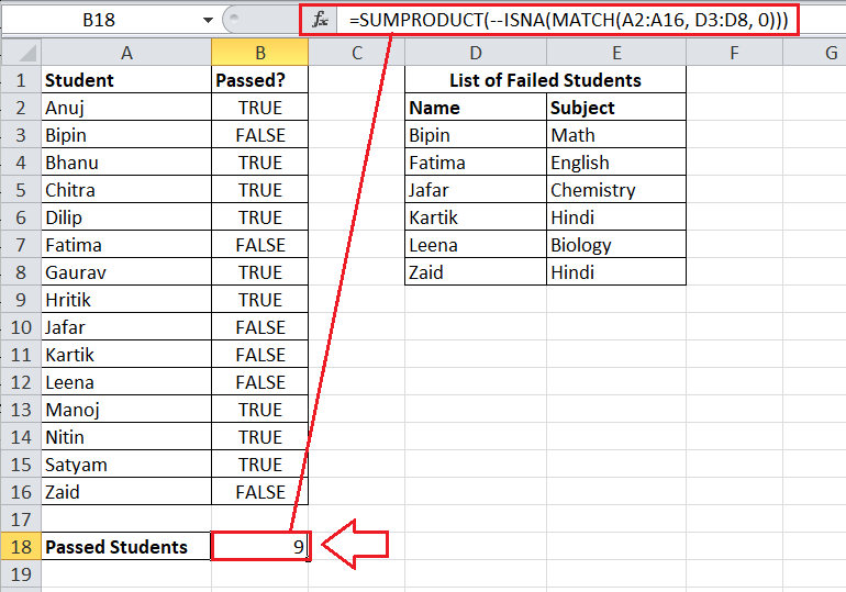
Here, the MATCH function returns nine #N/A errors as it does not find the names of 9 students in the list of failed students in column D. The ISNA function identifies the #N/A errors and returns TRUE for the corresponding values, which are then coerced into 1’s. Lastly, the SUMPRODUCT adds up all the 1’s and returns 9.
Important Points to Remember
- The ISNA function also includes blank (empty) cells from the given data set and returns FALSE accordingly because no #N/A error is found in empty cells.
- It is essential to note that the ISNA function in Excel does not help us locate the area where the #N/A error is present in our sheet. Instead, it only informs us whether there is a #N/A error in the given field or not.
- Instead of the IF-ISNA combination with VLOOKUP, we can also use the Excel IFNA function with the VLOOKUP to catch and handle #N/A errors and display a custom message. This helps make the formula shorter and easier to understand. However, the IFNA function is only available in Excel 2013 and higher versions.
- In Excel 365, 2021, and future versions, we can leverage the XLOOKUP function instead of the combined IF-ISNA-VLOOKUP. The XLOOKUP function can handle #N/A errors natively and show a custom message accordingly if needed.


