
Excel Hide Shortcut
MS Excel or Microsoft Excel is one of the most powerful spreadsheet software and has several distinct features. The hide feature in Excel is one of the useful features and helps users to manage vast amounts of data efficiently. The feature is very easy to use. It is used for both rows and columns accordingly.

This article discusses the Excel Hide feature and the process to use it using different shortcuts. The article includes the process for both hiding rows and columns.
What is the Hide feature in Excel Rows and Columns?
Excel Hide feature is one of the basic features, and it enables users to group the specific number of rows or columns and hides them temporarily. It mainly compresses the desired rows or columns within the Excel sheet. Users can unhide the rows/ columns whenever they need to see the details of the hidden rows/ columns.
Excel Hide feature is mainly used to hide rows/columns when the data is huge, and we want to hide unimportant data from the visible screen. The feature only hides data and does not change or affect results related to related rows/columns. The Hide feature is available in most Excel versions, including Excel 2007, 2010, 2013, 2016, 2019, and Office 365.
Hide Rows and Columns using Keyboard Shortcut
Excel has implemented several keyboard shortcuts to ease the use of Excel features. Users can perform most Excel tasks with shortcuts. Using the keyboard shortcuts reduces some steps and overall time of the working process. Thus, using keyboard shortcuts is the quickest and the most efficient way of performing most tasks in Excel. Thus, we must know the shortcut keys to hide rows and columns in Excel.
Since rows and columns the two different components of Excel, we use different shortcut keys to hide rows and columns:
For Hiding Row
The keyboard shortcut for hiding a row in Excel is “Ctrl + 9” without quotes. We need to follow the below steps to hide a row in Excel using a keyboard shortcut:
- First, we need to select a cell in the specific row that we want to hide. When we select or click on a cell, it becomes an active cell of the corresponding row.
- Next, we need to press and hold down the Ctrl key on the keyboard.
- Upon holding the Ctrl key, we need to press and release the key ‘9’. As soon as we press key 9 while holding the Ctrl key, the corresponding row is hidden from the visible screen.

For Hiding Column
The keyboard shortcut for hiding a column in Excel is “Ctrl + 0” without quotes. However, we must use the shortcut properly. We need to follow the below steps to hide a column in Excel using a keyboard shortcut:
- First, we need to select a cell in the specific column that we want to hide. When we select or click on a cell, it becomes an active cell of the corresponding column.
- Next, we need to press and hold down the Ctrl key on the keyboard.
- Upon holding the Ctrl key, we need to press and release the key ‘0’. As soon as we press the key 0 while holding the Ctrl key, the corresponding column is hidden from the visible screen.

Note: It should be noted that the keys ‘0 and 9’ must only be pressed from keyboard numbers. Using the respective keys from the number pad of the keyboard does not work.
Example
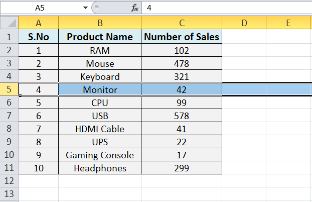
Suppose we have the following Excel sheet with some employees’ data. In the following Excel sheet, we want to hide the 5th and the column C using the keyboard shortcut. That means we need to hide a row and column in the same sheet.
We need to perform the following steps to hide the desired row and column in an example sheet:
- First, we must select a cell in a specific row or column that we need to hide accordingly. In our case, we select cell C5, as it is the cell in the 5th row and column C.

- Next, we need to press the shortcut Ctrl + 0 to hide the entire column C. Similarly, we need to press the shortcut Ctrl + 9 to hide the entire 5th row.
- Once we press the corresponding shortcut keys, the desired row and the column are hidden instantly. They are compressed between the rows and columns before and after them, respectively. After the desired row and column are hidden from the view, it looks like this:
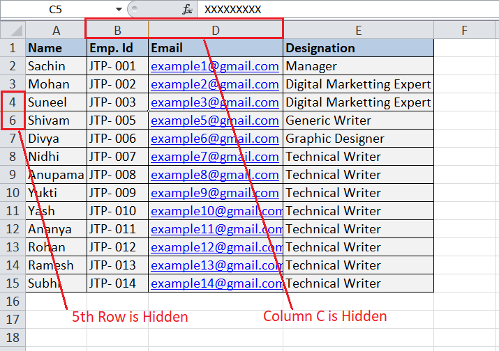
The above image shows a different sign (double lines or bold lines) in the respective headers (row header and column header) where the rows and columns are hidden.
That is how we can use the Excel Hide keyboard shortcut and hide a desired row or column.
Hide Rows and Columns using the Context Menu Shortcut
Another method to hide a row and column in Excel is to use the context menu. The context menu is accessed using the right-click directly on the row header or column header. Upon pressing the right-click on any headers, it displays some options, including the Hide option. However, it should be noted that the Context Menu only comes if the entire row/ column is selected when pressing the right-click button on the row/ column header.
For Hiding Row
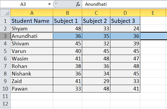
For hiding a row, we need to press the right-click on the row header. For example, suppose the following Excel data where we need to hide the 3rd row.

- First, we need to select any random cell in the 3rd row. In our case, we select cell B3. After selecting the cell, we need to press the shortcut Shift + Space to select the entire row. Alternately, we can directly click on the specific row header (such as 3 in our case) to select the entire row at once immediately.
- After selecting the row to be hidden, we must move the cursor to the corresponding row header and right-click on it. The right-click button triggers the context menu for the respective row, which looks like this:
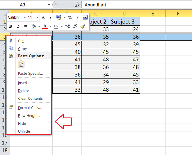
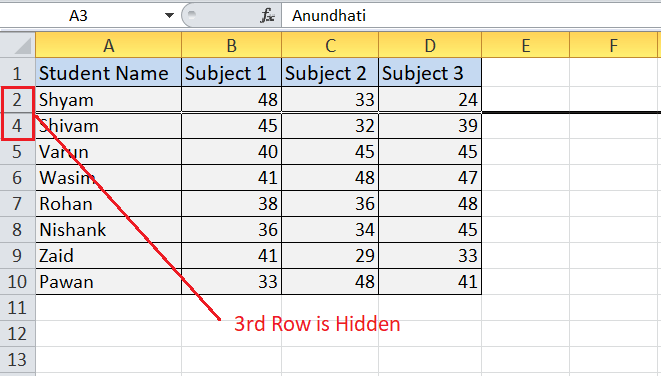
- Lastly, we need to select the option ‘Hide’ from the context menu list. As soon as we click the Hide option, the selected row is hidden between the rows before and after it (i.e., row 2nd and row 4th), as shown below:
For Hiding Column
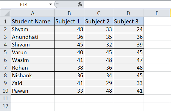
For hiding a column, we need to press the right-click on the column header. For example, suppose the following Excel data where we need to hide column B.
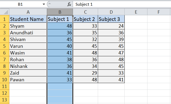
- First, we need to select the entire column B. We can select any cell of the desired column and the shortcut Ctrl + Space to select the entire column. Alternately, we can directly click on the specific column header (such as column B in our case) to select the entire column at once immediately.
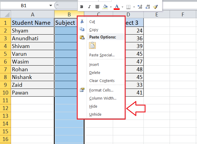
- After selecting the column to be hidden, we must move the cursor to the corresponding column header and right-click on it. The right-click button opens the context menu for the respective column, which looks like this:
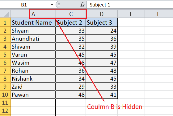
- Lastly, we need to select the option ‘Hide’ from the context menu list. As soon as we click the Hide option, the selected column is hidden between the columns before and after it (i.e., column A and column C), as shown below:
That is how we can use the Excel Hide shortcut from the context menu and hide a desired row or column.
Hide Rows and Columns using the Ribbon and its Shortcuts
The last method to hide the desired rows or columns includes the use of ribbon tabs and their respective shortcuts. This is a typical method to hide rows/ columns. The process is the same for both rows and columns. Let us discuss the steps:
- First, we need to select the specific row or column to hide. Let’s say we select the 5th row to hide in the following example sheet. To select the entire row/ column, we must click the row header/ column header, respectively. Since we are hiding the row, we click the row header of the 5th row.
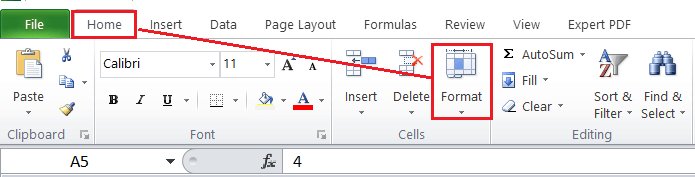
- Next, we need to navigate the Home tab and click the Format option, as shown below:
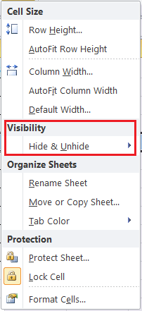
- After that, we need to select the option ‘Hide & Unhide’ under Visibility.
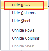
- Lastly, we must select the option ‘Hide Rows’ or ‘Hide Columns’ depending on what we want to hide. Since we have selected the 5th row to hide, we select the ‘Hide Rows’ option from the list. This will instantly hide the selected row, i.e. 5th row.
Apart from the steps mentioned above, we can also use the “Alt + H + O + U + R” shortcut without quotes. For this, we need to press the respective keys in series.
How to hide multiple rows/ columns in Excel?
Hiding multiple rows or columns is as easy as hiding an individual row or column. However, we must select all the corresponding rows/ columns before following any of the above methods. The easiest one is to use keyboard shortcut keys.
Let us understand the steps to hide multiple rows and columns in the same excel sheet with the help of an example:
Suppose we have the following Excel sheet where we need to hide columns ‘C & D’ and rows ‘3rd & 7th‘.
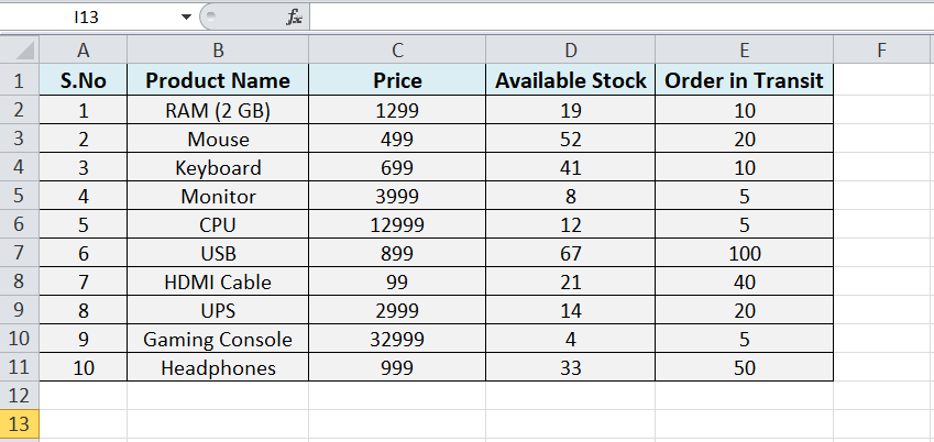
In this case, we will be hiding the adjacent columns and non-adjacent (separated) rows. This means we can hide both the adjacent and non-adjacent rows/ columns.
We need to perform the following steps to hide the corresponding rows/ columns in an example sheet:
- First, we need to select columns C and D to hide. To select the continuous columns, we can press and hold the Shift key and then click on the column header of the respective columns, i.e., columns C and D.
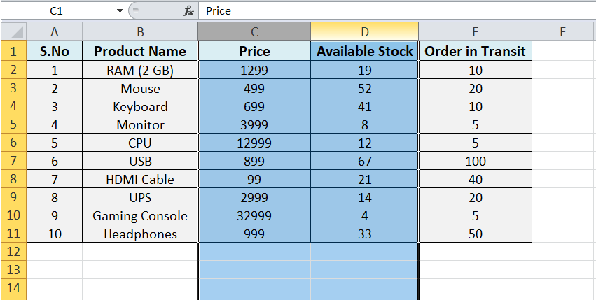
- After selecting the columns, we need to press the keyboard shortcut Ctrl + 0. As soon as we press the Excel Hide keyboard shortcut for columns, the corresponding columns will be hidden instantly. After hiding the columns, our example sheet looks like this:
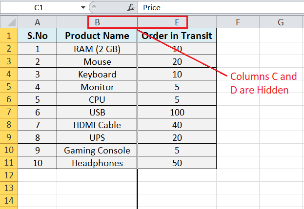
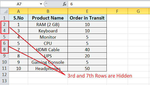
- Now, we need to hide the 3rd and 7th rows in the sheet. For this, we need to select both the respective rows. Since the rows are non-adjacent, we need to use the Ctrl button instead of the Shift button. We must press and hold the Ctrl key and then click on the row headers of the 3rd and 7th rows. This will select both the corresponding rows.
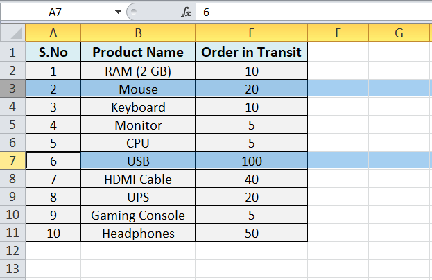
- After selecting the rows, we need to use the keyboard shortcut Ctrl + 9. This will hide the respective rows, i.e., the 3rd and 7th row. Now, our example sheet looks like this:
It should be noted here that we should use the Ctrl button to select non-adjacent rows/columns and the Shift button for adjacent rows/columns. In this way, we can hide multiple rows or columns, regardless of whether they are adjacent or non-adjacent.


