Excel group rows

When Excel has a worksheet with a lot and complex information, it is difficult to read and analyze the data. The user cannot easily analyze its data because of too much data inside it. Thus, Excel provides a way to organize the data in groups. These groups allow the users to expand and collapse the data of similar types of content. It creates a compact and understandable view of data.

This chapter will show you the usage of group rows in Excel that will help you to understand how to group rows in Excel. Learn this in the detailed description below in this chapter.

Group rows in Excel

There are thousands of rows and columns in an Excel worksheet that can contain data inside them. It is very difficult to extract meaningful data from it because whole data is not visible at once. Grouping is one of the best ways for the structured Excel worksheets that have column heading and does not have any blank row or column.

Excel users can use the process of automatic grouping or can manually group the rows in Excel. They can use any one of the methods to group the rows.

Why to group rows?

There are some reasons why an Excel user should use the Excel group feature to the rows.

• By grouping the rows, users can explore and collapse the rows in the worksheet.
• The data can be easily organized and analyzed.
• It can be a substitute for creating new sheets.

Group rows automatically

You can use this method to group the rows automatically if the Excel sheet contains just one level of information. This one is the fastest row to group the rows data automatically.

Follow the given steps below to group the rows automatically –

Step 1: We have taken the following set of data to group its rows data. Here, select a cell of one of the rows you want to group.

Select any cell you want to group.+

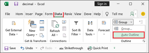
Step 2: Now, go to the Data tab on the Excel ribbon inside which click the Group option resides in the Outline section.

Step 3: Inside the Group dropdown button, choose Auto Outline to automatically group the selected data.

For this method, that’s all.

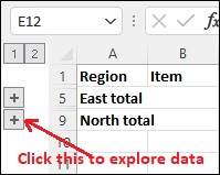
Step 4: Your data is grouped automatically here. You can now explore the visualization option to see the complete data that is grouped.

Earlier, you can see that the whole data was shown. You have to scroll down to see the data. But now, the data is grouped in different rows that are now easy to read and analyze.

How to group rows manually

When your Excel worksheets contain more than one level of information, the above Auto Outline feature may not work to group the data correctly. Thus, you have to try another method to get this done. You can manually group the rows instead of Auto Outline. To do this, perform the following steps with your data.

“Before using this method, make sure your sheet does not contain any hidden row or column. Otherwise, the data may not be grouped correctly.”

Method 1: Create outer groups (level 1)

Step 1: We have taken the following data to group together that is parted into multiple dataset sections.

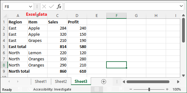
Step 2: Select a subset of data to group and navigate to the Data tab. We have selected A2 to D4 for row 5, i.e., East Subtotal.

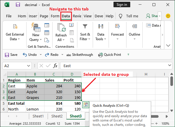
Step 3: In the Data tab, click the Group inside the Outline group section.

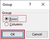
Step 4: A small popup panel will open on which select the Rows radio button and click OK.

Step 5: You will see a vertical bar inserted on the left side of the sheet. It contains a visualization action button to explore the grouped data.

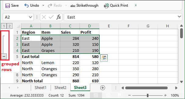
Currently, the grouped data is fully visible.

Step 6: Click this – sign inside the square box on the left side of the sheet to hide the grouped data. The data will show you like below:

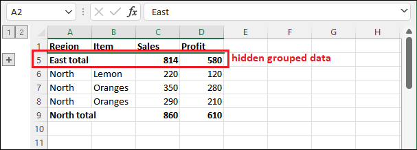
You can now click the + sign to explore and see complete data. In the same way, users can create as many as groups they want or need.

Tip: To make the grouping process faster, select the targeted data and press the Shift + Alt + Right Arrow shortcut key to group data together manually.

Step 7: We have grouped one more dataset (for the north region) in this sheet by following the same steps as above.

Ungroup the grouped rows

You may also need to ungroup the grouped rows. You can do it too by using Ungroup feature of Excel that is available with the Group feature. Use the following steps to ungroup the rows.

Step 1: We will use the above data that is grouped into two groups. One for East total and another for North total.

Step 2: Firstly, explore the data by clicking the + sign corresponding to make the data grouped data visible.

Step 3: Now, select the grouped data cells to which you want to ungroup and then navigate to the Data tab.

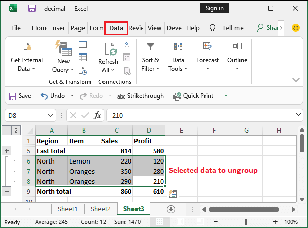
Step 4: In the Data tab, click the Ungroup inside the Outline group section.

Step 5: A small popup panel will open on which select Row radio button to ungroup the rows and click OK.

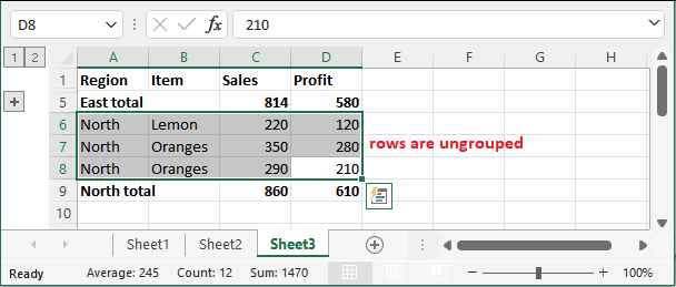
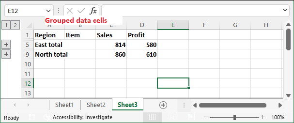
Step 6: Your selected rows are now ungrouped, as you can see in the below screenshot.

In the same way, you can ungroup the other data by following these steps one by one.

Method 2: Create nested groups

Excel allows its users to create an outline that consists up to eight levels. We will describe creating the nested groups by taking an example. For creating the nested group, we have taken the following dataset:

Create outer groups (level 1)

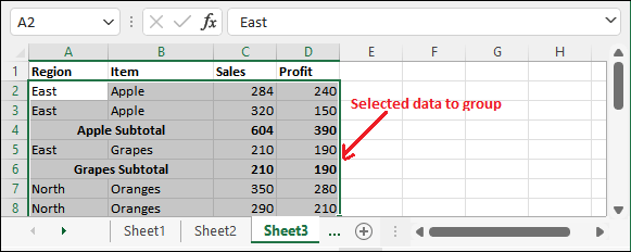
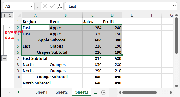
Step 1: Select the dataset along with the intermediate summary rows and detail rows. We have selected data for East region for both Apple, grapes, and Oranges with subtotal.

Step 2: Now, navigate to the Data tab in Excel ribbon and click the Group option inside the Outline group section.

Step 3: A small popup panel will open on which select the Rows radio button and click OK.

Step 4: Your selected rows will be grouped together and you will see a visualization icon on the left side of the Excel sheet screen.

A user can explore and collapse the grouped rows using this visualization icon. In the same way, you can as many you want outer groups.

Create nested groups (level 2)

We will perform the following steps described below to elaborate the nested groups. The data will be the same as we used for the above example with some small changes.

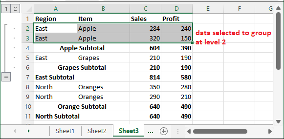
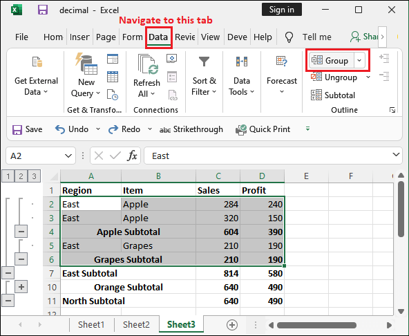
Step 1: Select the dataset along with the intermediate summary rows and detail rows. For example, we will select East region data for both Apple and Oranges with subtotal.

Step 2: Now, go to the Data tab and click the Group option present at the end of the ribbon.

Step 3: Select the Rows radio button to group the data by row.

Step 4: You can see that the data is grouped for the East region. Now, move to the next level.

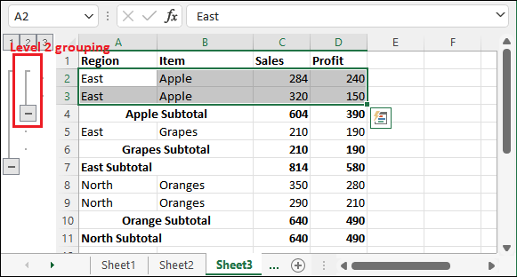
Step 5: Now, select only row 2 and 3 for Apple in East region.

Step 6: Now, repeat step 2 to step 4 again to group the selected rows data. The data row 2 and 3 will be grouped like as shown below.

Step 7: Select row 5 to group the grapes for East region for level 2 grouping.

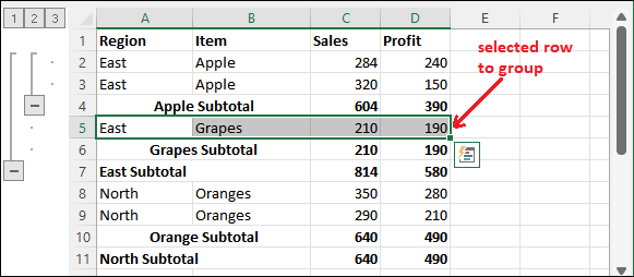
Step 8: Now, repeat step 2 to step 4 again to group the selected rows data. The row 5 will be grouped like as shown below inside the outer group.

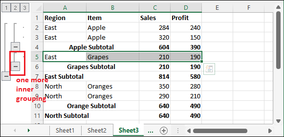
Step 9: In the same way, we will group the North region data for oranges. At the end, after the whole data grouping, the data table will look like as below.

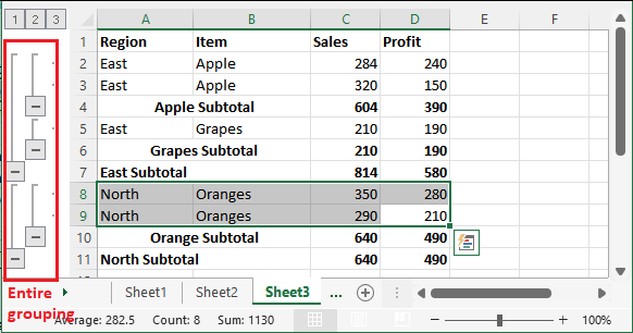
In this way, an Excel user can group the data stored in an Excel sheet and analyze it easily. You can expand and collapse the data rows to see the data however you want.

Ungroup the grouped rows

You may also need to ungroup the rows that you have grouped earlier. You can do it too by using Ungroup or Clear Outline feature of Excel that is available with the Group feature.

• Use the Ungroup option if you want to only one or two groups, not all.
• In case if you want to ungroup the entire sheet rows data, use the Clear Outline option to ungroup all grouped rows at once.

Ungrouped all grouped rows at once

This method is useful when multiple rows grouping in an Excel sheet and you want to ungroup all of them in one go. You can follow these steps to ungroup the rows.

Use the following steps to ungroup all grouped rows at once.

Step 1: Open the Excel file that contains the grouped rows. We have the following sheet with grouped rows.

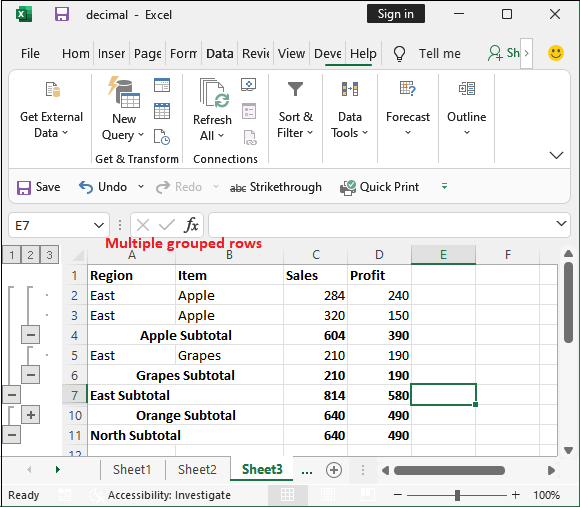
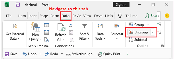
Step 2: Navigate to the Data tab and click the Ungroup dropdown option in the ribbon.

Step 3: Inside the Ungroup dropdown list, choose Clear Outline to ungroup all the grouped rows at once.

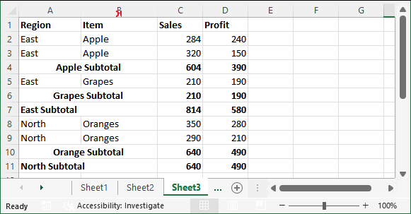
Step 4: You will see that all rows are ungrouped now only in one click.

Ungrouped the specific grouped row

This method is useful when you want to ungroup any specific grouped row instead of the entire sheet.

Use the following steps if you want to ungroup the rows one by one or a specific grouped row.

Step 1: We will use the above data grouped in outer and inner groups for East total and another for North total.

Here, we will ungroup the outer grouped row for East subtotal.

Step 2: So, select row 2 to row 6 and navigate to the Data tab, where you will see the Ungroup option inside the Outline section.

Step 3: Click this Ungroup option to ungroup the selected rows.

Step 4: A small popup panel will open on which select Row radio button to ungroup the rows and click OK.

Step 5: You will see that the outer grouped rows are ungrouped and inner grouping is still there.

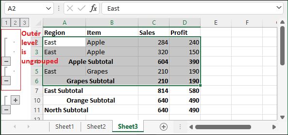
Your selected row has been ungrouped (outer grouped row) now ungrouped as you can see in the above screenshot.

In the same way, you can ungroup the other data by following these steps one by one.

---