
Excel Filter Shortcut
MS Excel or Microsoft Excel is a powerful spreadsheet software with numerous distinct features. One such essential feature is a Filter in Excel. In particular, the filter’s primary function is to highlight only the crucial entries of a dataset. The filter feature is mainly helpful when working with vast amounts of data because it helps display required data by eliminating the unnecessary entries temporarily from the display area.
When applying the filter in Excel, we select the entries to be visible and hidden based on specific rules according to our needs. Furthermore, it is usually a multi-step process. Therefore, we must know different shortcuts to filter the data quickly and save our time to some extent. In this article, we discuss some Excel Filter Shortcuts that will be useful to find the desired data quickly as per our need and increase the overall work productivity.

Filter Shortcuts in Excel
The following are some essential shortcuts for applying filters on Excel data sets:
- By using the keyboard shortcut keys
- By using the Filter shortcut under Data
- By using the Filter shortcut under ‘Sort and Filter’
Let us now discuss each method in detail:
By using the keyboard shortcut keys
Excel supports an extensive range of keyboard shortcuts to help us cut the working time and increase the speed. The keyboard shortcuts are best and the most effective for manipulating the data using filters in Excel.
Following are some frequently used filtering options with keyboard shortcuts:
Create Filters
Creating a filter is the first step of filtering the data. We need to select a cell inside our data range and then use the keyboard shortcut Ctrl + T or Ctrl + L. After pressing the shortcut, Excel will display a dialogue box asking us whether our data includes headers or not. Once we have selected the options, we need to click the OK button. By doing this, Excel will transform the data into a table and enable filters.
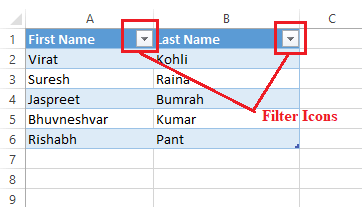
For example, let us take the following data set where we have headers (First Name, Last Name):

When we select a cell A2, and we press the shortcut key Ctrl + T, we get the dialogue box:

Since we have the headers, we select the checkmark. After clicking the OK button, we get the filter icons next to the text (names) of the headers. It looks like this:
Turn Filters On/ Off
Another shortcut to create filters in Excel involves the use of shortcut Ctrl + Shift + L. Unlike the previous shortcut, this particular shortcut requires headers in columns because it does not allow us to choose whether we have headers or not. Instead, it automatically considers that we have headers in our data. Apart from this, this shortcut (Ctrl + Shift + L) does not format the data. The only advantage of using this shortcut to create filters is that we can also turn off the filters using the same shortcut.
Since our example data set consists of headers, we can use the shortcut Ctrl + Shift + L. After using the shortcut, we get the following results:

When we again press the shortcut keys, the filter icons are removed from the headers. However, our filtering options and filtered data will also be used. This way, we can turn the filters on and off in Excel.
Access Filter Drop-Down Menu
Once the filter icon (also called the filter drop-down menu) is enabled, we need to click it to access the filter drop-down menu. To click it, we can either use mouse buttons or keyboard shortcuts. When using keyboard shortcuts, we must first move the cursor to the column header using the arrow keys and press the Left Alt + Down Arrow (?) key. This will display the filter menu and its options.

Select Menu Items with Arrow Keys
Once the filter menu is opened, we can use the arrow keys on the keyboard to navigate the options within the menu. We can select left, right, up, down commands using the arrow keys ← → ↑ ↓, respectively. Additionally, we can also use the Tab key to move forward and Shift + Tab to move backward.
Drop-Down Menu Shortcuts
Although we can navigate the menu items using the Tab key or the arrow keys, we have better options. Excel makes it even easier to use keyboard shortcuts with the menu items. We can press some specific characters after opening the filter menu using the left Alt + Down Arrow Key.
The following keys can be used to perform the corresponding actions:
- S: We can press the ‘S’ key to sort the data in ascending order, i.e., A to Z.
- O: We can press the ‘O’ key to sort the data in descending order, i.e., Z to A.
- T: We can press the ‘T’ key to sort the data by color.
- C: We can press the ‘C’ key to clear the filter.
- I: We can press the ‘I’ key to filter the data by color.
- F: We can press the ‘F’ key to apply text filters or display the text, number, or date filters sub-menu.
- E: We can press the ‘E’ key to access the search/ text box.
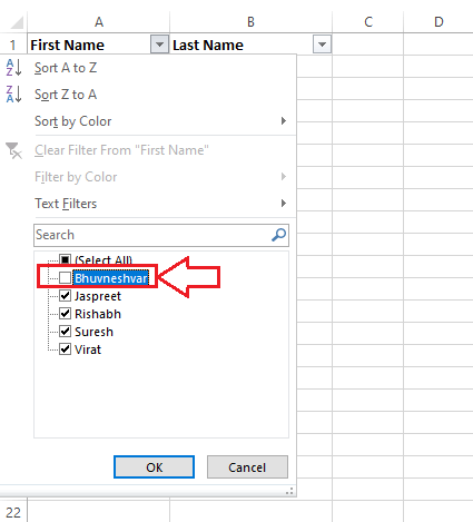
Check/ Uncheck Filter Items
The unique filtered entities are displayed under the search box, lying at the bottom of the filter menu. We need to select/ deselect the entities to filter the data as required. For this, we must check/ uncheck respective checkboxes. To check or uncheck the desired box, we need to move our cursor to that particular item and then press the Spacebar on the keyboard. The Spacebar key can be used to check and uncheck the desired items from within the filter items.
Once we are done with checking boxes, we need to press the Enter key on the keyboard to confirm and apply filtering options.
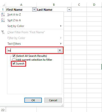
Access Search Box in Filter Menu
The search box feature was added in Excel 2010 and is still present in the latest version. This feature helps us locate the desired item from the list without scrolling through the entire list of items. It can be easily accessed by pressing the keyboard key. But, we must have already opened the filter menu from the corresponding header by using Left Alt + Down Arrow Key.
If the filter menu is opened, we must press the letter ‘E’ on the keyboard. This will directly move the cursor to the search box, and we will be able to type whatever we need to select from the list. This way, we can quickly filter the data as per our needs.
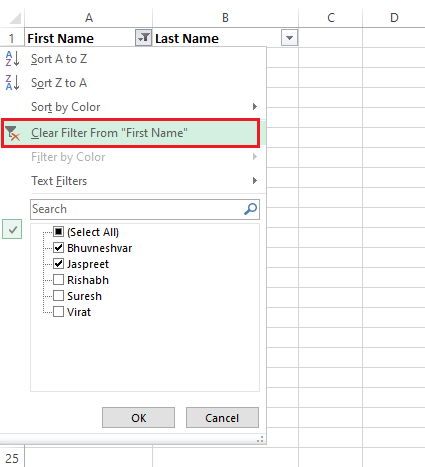
Clear All Filters in Column
If the filter is applied and we want to remove it, we can use the clear filter option from the list. First, we need to open the filter menu for the corresponding column header. Once the filter menu is displayed, we must press the letter ‘C’ on the keyboard. This will instantly clear all the filters from the column. This way, we can remove filters from other columns as well.
Clear All Filters at Once
Although the above method can be used to clear filters from each specific column one by one, we can also use another shortcut to clear filters from all columns at once. That means, if we want to remove the filter from all the columns instead of one, we can use this method. According to this method, we need to press the Alt key, the letter A, and then the letter C in sequence one after another, i.e., Alt >> A >> C.
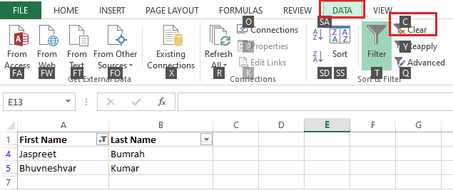
The shortcut here typically goes through Data > Clear Filter in the ribbon. This will clear all the filters from the current worksheet.
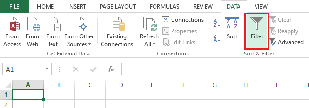
By using the Filter shortcut under Data Tab
Another method to use the filter in Excel includes the use of Filter shortcut tile. It can be accessed by navigating through the Data tab inside the ribbon. It looks like this:
For example, suppose we have the following excel sheet:

Let us apply a filter using this shortcut:
- First, we need to select any specific cell or the range of data to apply a filter. After that, we must go to Data > Filter.
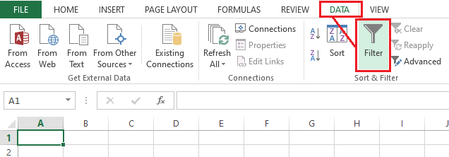
- After we click the Filter option, we will see that the filter is applied to the selected cell or data range. Excel enables filter icons in corresponding columns, which looks like this:

- We need to click the filter icon or the filter drop-down menu icon to access the menu items.
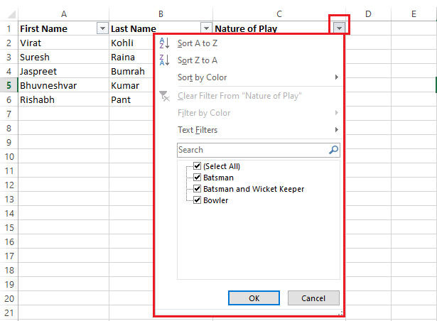
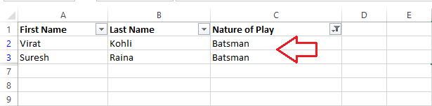
Suppose we only want to display the names of the batsman. For this, we need to select the checkbox ‘Batsman’ and click the OK button.

We will only get the names of all those players who are batsmen, such as:
To disable the filters and get all the data back, we can click the filter tile again from the ribbon.
Note: It must be noted that the filter option in Excel does not delete the entries. Instead, it just makes the entries visible and hidden as per the applied rules by the user.
By using the Filter shortcut under ‘Sort and Filter’
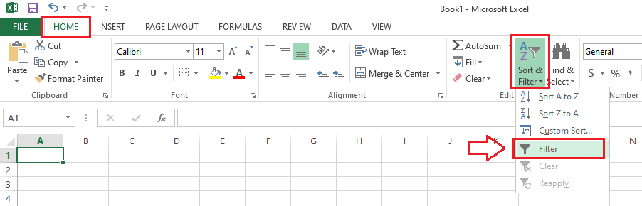
MS Excel offers one more shortcut to apply the filter in our Excel sheet. The shortcut can be easily accessed from the right side of the ribbon under the Editing section of the Home tab. It is named ‘Sort & Filter’. However, we must choose ‘Filter’ after clicking on the ‘Sort & Filter’ shortcut. It looks like this:

Let us now try this method and apply the filter in the following Excel sheet:
- First, we need to select the columns or entire data range where we want to apply the filters. Next, we must navigate to the Home > Sort & Filter > Filter.
- After clicking the Filter option from the list, we will see that the selected area has new filter icons next to text written in the columns. It looks like the below image:
- After that, we need to click on the desired filter icon to expand the filter menu.
- Once the filter menu is displayed, we can select the entities to make them visible or hidden accordingly. Suppose we want to highlight only the bowler names in our excel sheet. For this, we need to select the check box associated with the text ‘Bowler’ and deselect all other checkboxes. Lastly, we must click on the OK button.

By doing this, we will only get the names of bowlers from our data set, such as:

That is how we can filter data in Excel using the Excel Filter shortcuts.


