
Excel CEILING Function
Rounding is a useful Excel feature that helps you in situations where you don’t require an exact answer. It is a technique that fetches an approximate number with the expected level of accuracy. In simple terms, rounding a number eliminates the smallest significant digits, making the value shorter but holding it close to the actual number. Microsoft Excel provides various built-in rounding functions, and one of them is the CEILING function.
This tutorial will cover the definition of Excel CEILING Function, its syntax, parameters, return type, steps to implement CEILING function in your worksheet, different examples to round decimal numbers to integers, round a number to nearest multiple, and many more!
What is CEILING Function?
The CEILING function in Excel rounds a given number up to the nearest multiple of significance. It has the same syntax as the FLOOR function, but the FLOOR function is used to round down the number, whereas the CEILING function rounds up the number.
This function rounds a number up to the specified multiple (provided in the Significance parameter). No rounding happens if the specified number is already an exact multiple, and this function returns the original number. The multiple to utilize for rounding any number is supplied as the significance parameter.
This function accepts two parameters, i.e., the number and the Significance. The Number argument represents the numeric value you want to round up to an exact multiple. The significance parameter represents the multiple to which the specified number should be rounded up.
The CEILING Function is categorized under Math/Trig Function. It works similarly as the FLOOR or MROUND function, but unlike FLLOR or MROUND, which rounds down to the nearest multiple or rounds to nearest multiple, CEILING always rounds up.
Note: The Excel CEILING function is officially documented as compatibility function replaced by Excel CEILING.MATH and CEILING.PRECISE.
Syntax
Parameter
- Number (required) – This parameter represents the number that should be rounded.
- Significance (required) – This parameter represents multiple to use when rounding. The sign much matches the number. So if the number is negative, the Significance must also be negative.
Return
The Excel CEILING function returns a number rounding it up to the specified multiple.
Rules for Excel CEILING Function
The CEILING is a built-in function in Excel that works based on some pre-defined rounding rules that generally rounds up the number away from 0. Before implementing the function in your worksheets, have a look at the following rules:
- If both the parameters (number and significance) are positive, the given number is rounded up. For instance, the number argument is 12, whereas the significance is 5, so the number 12 is rounded up to 15. Refer to the image given below:

- If the parameter number is positive and the parameter significance is negative, the CEILING function returns the #NUM error. Refer to the below image.

- If the number argument is negative and the significance argument is positive, the number is rounded up, towards zero. Refer to the below image.

- If both the parameters (number and significance) are negative, the given number is rounded down. Refer to the below image.

Examples
Example 1: Using the CEILING function round up the values to the given multiple.
| Number | Significance |
|---|---|
| 52 | 3 |
| 54 | 5 |
| 21 | 10 |
| 130 | 12 |
| 123 | -3 |
| 12 | 10 |
Follow the below given steps to round up the above numbers using the CEILING function:
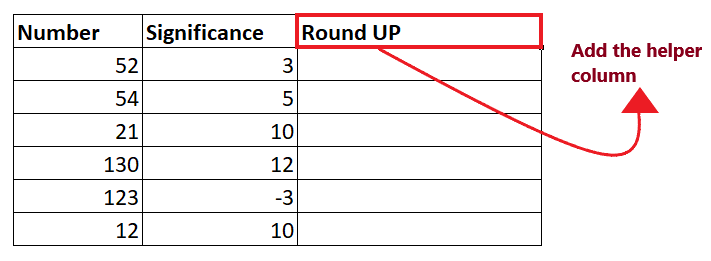
Step 1: Insert the helper columns
We will add the helper column named with ‘Round up’ in cell E3. In this column, we will use the CEILING function to round up the numbers down to the specified Significance value.
Refer to the given below image:
STEP 2: Implement the CEILING Function
- Excel provides an inbuilt function CEILING that helps to round a given number up, to the nearest multiple of a specified significance.
- In the “Round up” helper column, start the formula with the equal sign (=) and type the CEILING function. So our formula becomes: =CEILING(

STEP 3: Insert the CEILING Parameters
- At first it will ask for the number parameter. Here specify the number that you want to round of. In our case, we will refer to cell C4. So our formula becomes: = CEILING (C4,

- Next, supply the significance parameter. In our case, we will refer to cell D4. Therefore, our formula becomes: = CEILING (C4, D4)

STEP 4: Excel will return the output
- Once you have typed the formula, press the Enter button to complete it.
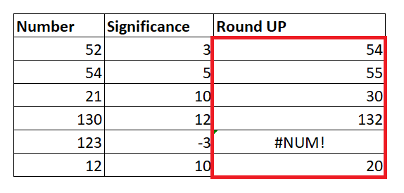
- The above formula will return a number after rounding it down to 3. Since the given number is 52 (multiple of 3) will return 54 as shown in the below image.

STEP 5: Copy the formula across all the cells
- Select the cell where you have typed the formula. Take your mouse cursor towards the end of the rectangular box. You will notice the cursor will change into a small thin black cross. Drag it down to the cells to which you want to auto-fill the CEILING formula.
- The formula will get copied where the absolute cell reference values will change and you will get the output for each cell.
You will have the following output.
Example 2: Round the given pricing up to end with .99
| Pricing |
|---|
| 8952 |
| 2154 |
| 231 |
| 1390 |
| 1293 |
| 1212 |
You can also use the Excel CEILING function to set the pricing after currency conversion, or getting discounts, etc. To round up the pricing to end with .99, follow the below-given steps:
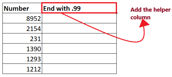
Step 1: Insert the helper columns
We will add the helper column helper with ‘End with .99’ in cell D3. In this column, we will use the CEILING function to round up the pricing so it ends with .99.
Refer to the given below image:
STEP 2: Implement the CEILING Function
- Excel provides an inbuilt function CEILING that helps to round up a given number to the nearest multiple of a specified significance.
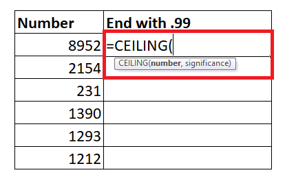
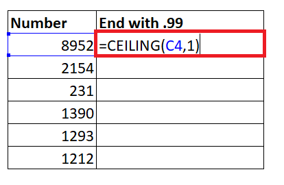
- In the “‘End with .99′” helper column, start the formula with the equal sign (=) and type the CEILING function. So our formula becomes: = CEILING (
STEP 3: Insert the CEILING Parameters
- At first it will ask for the number parameter. Here specify the number that you want to round of. In our case, we will refer to cell C3. So our formula becomes: = CEILING (C4,

- Next, supply the significance parameter. In the question itself the significance is given as 1. Therefore, our formula becomes: = CEILING (C4, 1)
- Then subtract 1 cent, to return a price like 341.99, 54.99, 69.99, etc. Our formula becomes: = CEILING (C4, 1) – 0.01

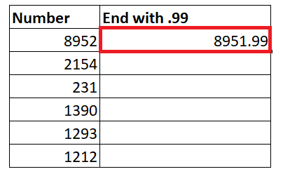
STEP 4: Excel will return the output
- Once, you have typed the formula, press the Enter button to complete it.
- The above formula will return a number ending with .99 after it rounding to 1. You will have the following output:
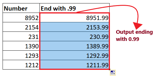
STEP 5: Copy the formula across all the cells
- Select the cell where you have typed the formula. Take your mouse cursor towards the end of the rectangular box. You will notice the cursor will change into a small thin black cross. Drag it down to the cells to which you want to auto-fill the CEILING formula.
- The formula will get copied where the absolute cell reference values will change and you will get the round output for each cell.
You will have the following output.
Example 3: Using the Excel CEILING function round up the given time in the Time column to nearest 15 minutes
The Excel CEILING function comprehends the time formats, and therefore can be used to round up the time to the specified multiple. To round up the Time to nearest 15 minutes, follow the below given steps:
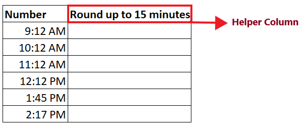
Step 1: Insert the helper columns
We will add the helper column helper with ‘Round up to 15 minutes’ in cell D3. In this column, we will use the CEILING function to round up the time to nearest 15 minutes.
Refer to the given below image:
STEP 2: Implement the CEILING Function
- Excel provides an inbuilt function CEILING that helps to round up the given number to the nearest multiple of a specified significance.
- In the ‘nearest 15 minutes’ helper column, start the formula with the equal sign (=) and type the CEILING function. So our formula becomes: = CEILING (

STEP 3: Insert the CEILING Parameters
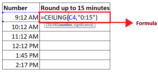
- At first it will ask for the number parameter. Here specify the number that you want to round of. In our case, we will refer to cell C4. So our formula becomes: = CEILING(C4,
- Next, supply the significance parameter. In the question itself the significance is given as nearest 15 minutes. Time values can also be entered in the Significance text like “1:16”. So here we will pass ‘0:15’. Therefore, our formula becomes: = CEILING (C4, “0:15”)
STEP 4: Excel will return the output
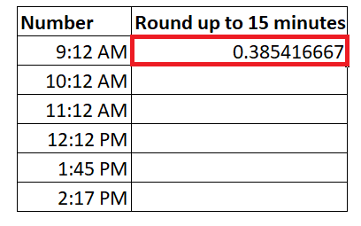
- Once, you have typed the formula, press the Enter button to complete it.
- The above formula will return a number after it rounding to “0:15”. You will have the following output:
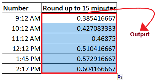
STEP 5: Copy the formula across all the cells
- Select the cell where you have typed the formula. Take your mouse cursor towards the end of the rectangular box. You will notice the cursor will change into a small thin black cross. Drag it down to the cells to which you want to auto-fill the CEILING formula.
- The formula will get copied where the absolute cell reference values will change and you will get the output for each cell.
You will have the following output.
Other rounding functions in Excel
- You can implement the Excel ROUND function when you want to round the numbers normally.
- You can implement the Excel MROUND function when you want to round the numbers to the nearest multiple.
- You can implement the Excel ROUNDDOWN function when you want to round down to the nearest specified place.
- You can implement the Excel ROUNDUP function to round up to the nearest specified place.
- You can implement the Excel FLOOR function to round down the given number to the nearest specified multiple.
- You can implement the Excel INT function to round down the given number and return an integer only.
- You can implement the Excel TRUNC function to truncate decimal places.


