
Excel AVERAGE() Function
MS Excel is a widely popular spreadsheet program that comes inbuilt with the Microsoft Office package. Excel has a wide range of supported functions to help us perform operations on the data within the sheet. It has more than 400 functions, and the AVERAGE() function is one of the most used functions in Excel.
In this article, we discuss the process of using the Excel AVERAGE() function, including its syntax and examples.
What is the AVERAGE Function in Excel?
The AVERAGE function is one of the popular built-in functions in Excel. It is found in a category of Excel Statistical Functions. The AVERAGE function is typically used to retrieve the average value or arithmetic mean from the supplied range or cells of numerical values. The function can accept series of numbers and calculate the arithmetic mean of the supplied arguments accordingly.
The AVERAGE function can be easily used as a typical worksheet function in Excel. This means that Excel allows us to apply the AVERAGE function as part of a formula to one or more desired cells within the sheet. The AVERAGE function is inbuilt in all the versions of MS Excel, including the latest Office 365, Excel 2019, Excel 2016, Excel 2013, etc.
The AVERAGE function is useful in financial analysis and can determine the mean value (average) of the series of numbers in many conditions. For instance, we can calculate the average sales of any product for the previous six months or more in a business.
Syntax
The following is the syntax of the AVERAGE function in Excel:
In this syntax, we can identify the numbers using the set of one or more numeric values, named range, arrays, a reference to the particular cell, or a range of numbers.
Arguments or Parameters
The AVERAGE function must be used with at least one argument, meaning that one argument is compulsory to be supplied to this function. Apart from this, the rest of the arguments are optional. They can be either supplied or ignored to the AVERAGE function based on the requirements.
The AVERAGE function has the following arguments:
- Compulsory Argument: number1 is the required argument or parameter in the AVERAGE function. It must be supplied to the function as the first number or cell reference containing the numerical values of the range we want to calculate the average.
- Optional Argument: number2 and other subsequent arguments are optional and can be supplied the same way as the compulsory argument. However, they are the additional numbers, cell references, or a range we want to calculate the average.
In older versions of Excel, such as Excel 2003 and earlier, the AVERAGE function accepts up to a maximum of 30 arguments. However, the limit was increased in later versions. Thus, the later versions (Excel 2007 and higher) allow us to use up to 255 individual arguments in the AVERAGE function. Moreover, we can define each argument as an array of values or a range of cells, further containing many other values.
Returns
The AVERAGE function in Excel returns the average numeric value from the selected/ supplied set of data cells/ ranges of numbers.
How to use AVERAGE Function in Excel?
The AVERAGE function is one of the most basic and easy-to-use built-in functions. We can use this particular function as a usual worksheet function in an Excel sheet. This determines that we can apply the AVERAGE function as a part of the formula in one or more desired cells in the sheet.
To use the AVERAGE function in its simplest form within the Excel sheet, we must start typing it in the desired cell and provide random numeric values as arguments. For example:
In this example, the AVERAGE function returns the value 2 as an output because it is the average value of all the three supplied arguments. However, it is rarely seen that we need to deal with the values directly in the function as arguments. Instead, we typically use operations on values stored in cells or ranges. In such a case, we need to perform the below steps to use the AVERAGE function and calculate the average value from the specified or selected range of cells/ data:
- First, we must choose a specific cell to store an average value and then start typing the AVERAGE function ‘=AVERAGE(‘ in it without the quotation marks.
- After typing the opening parenthesis, we must select all the effective cells or range of values for which we want to calculate the resultant average value. We can use the mouse drag feature to select the desired cells/ ranges.
- After selecting all the desired cells/ ranges, we must close the function by typing the ending parenthesis ‘)’ without the quotation marks.
- Finally, we must press the Enter key to register an average value in a selected cell.
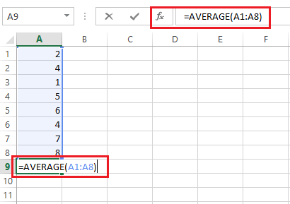
Suppose we have the following excel sheet, and we want to calculate the average value of the values stored in column A. Since we have effective values in the range of cells from cell A1 to cell A8, we apply the AVERAGE function only for this specific range. If we consider cell A9 as the result cell, we use the AVERAGE function in cell A9 like in the following image:
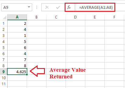
Lastly, we press the Enter key, and the function returns the average value for the specified range in a result cell:
Let us now understand the different use cases of the AVERAGE function with the help of the following examples:
Excel AVERAGE Function Examples
The following examples discuss the process on how we can use the AVERAGE function in different ways:
Example 1: Calculating the Average Marks
We can calculate the arithmetic mean or average of some values or marks written in an Excel sheet. For this, we need to select the range of marks for which we want to find out the results and apply the AVERAGE function on it. We can select the result cell accordingly before we apply the AVERAGE function.
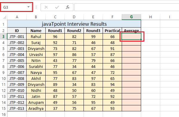
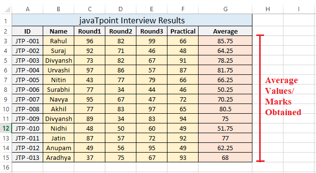
For instance, let us consider the following Excel sheet with some marks given to employees in an interview. We want to calculate the average marks achieved by each employee.

We can perform the following steps to obtain a mean or average marks for each employee:
- First, we need to calculate the average marks of the first employee. For this, we must apply the AVERAGE function for the range of C3:F3 in a result cell G3. Thus, we select the result cell G3.
- Next, we enter the AVERAGE function in a result cell and select the reference cells or range with marks like the following image:
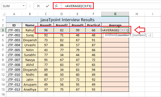
- After that, we need to press the Enter key to retrieve the average marks for the first employee in the example list.

- Once we have successfully obtained the average marks for the first employee, we can drag the particular cell to the bottom of the result cells, which will apply the corresponding formula in all the result cells. For this, we can use a drag holder from the bottom-right corner of the specific cell.

This will quickly provide the average marks for all the employees on the list.
Although we can apply the AVERAGE function in all the result cells one by one, it will take more time. Thus, dragging a cell is the better solution.
Example 2: Calculating the Average Sales
The AVERAGE function is used in most financial sectors to find the average sales and total average revenue for a specific period. This function makes calculating average sales or revenue easy when related data is stored in an Excel sheet. The main advantage of using the AVERAGE function in the excel sheet is that we can update the data whenever required and get the corresponding average result in real-time.
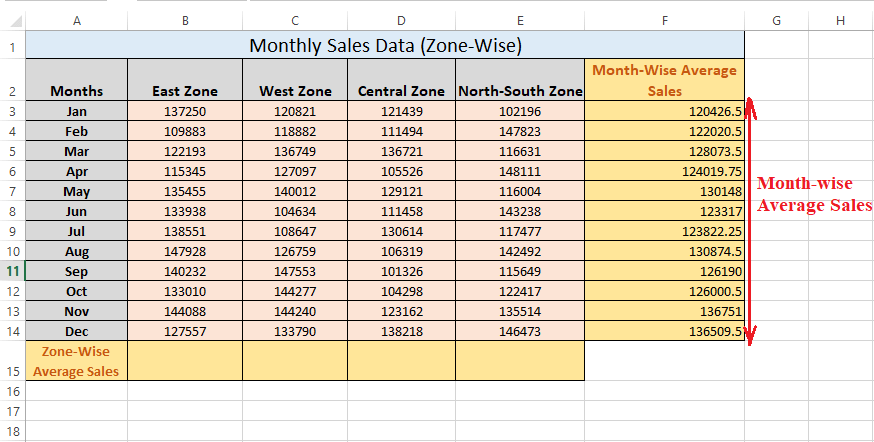
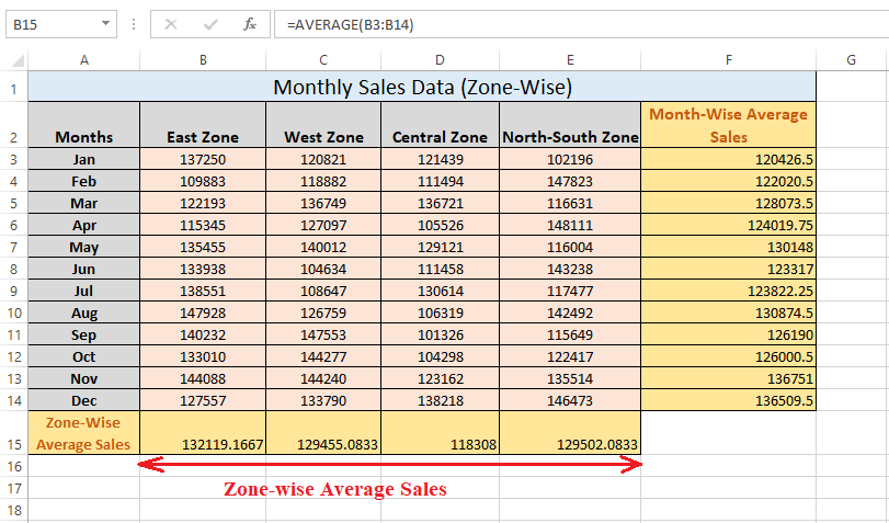
For instance, let us consider the following Excel sheet with some monthly sales data for any company. The overall sales data is divided into four different zones. Now, we want to calculate the average sales for each month and each zone.
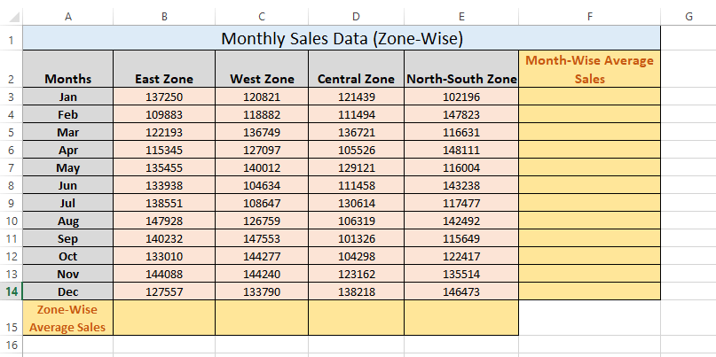
We can perform the following steps to obtain a mean or average sales for each month and each zone:
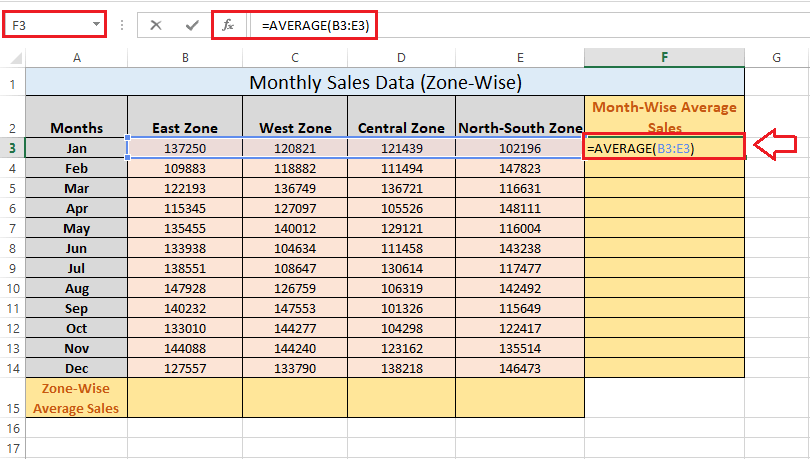
- First, we calculate the average sales for January month by applying the AVERAGE function to the sales data of January month. For this, we select the result cell F3 and enter the AVERAGE function for the range of data in B3:E3, as shown below:
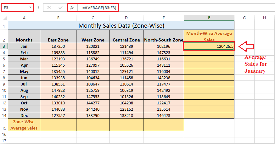
- After pressing the Enter key, we retrieve the average sales for January month.
- Similarly, we can apply the AVERAGE function to get the average sales for other months. However, we typically drag the result cell to the bottom of the result cells, and the corresponding data is supplied to the AVERAGE function for each month accordingly.

This provides the average sales for each month instantly, as shown below:
- Next, we need to calculate the average sales for each zone. For this, we apply the AVERAGE function to the result cell B15 for the range B3:B14.
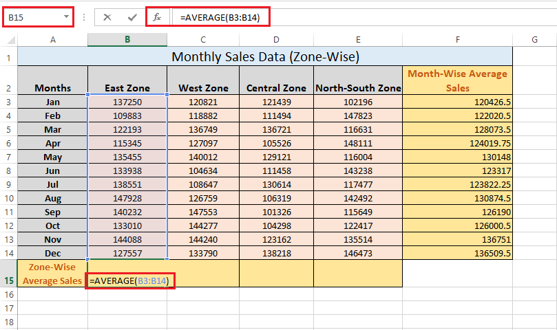
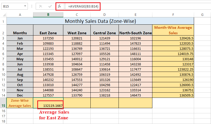
Next, we press the Enter key to get the calculated value. By doing this, we only calculate the average sales for the east zone.
- Lastly, we drag the result cell B15 to other cells C15, D15, and E15 using the mouse.
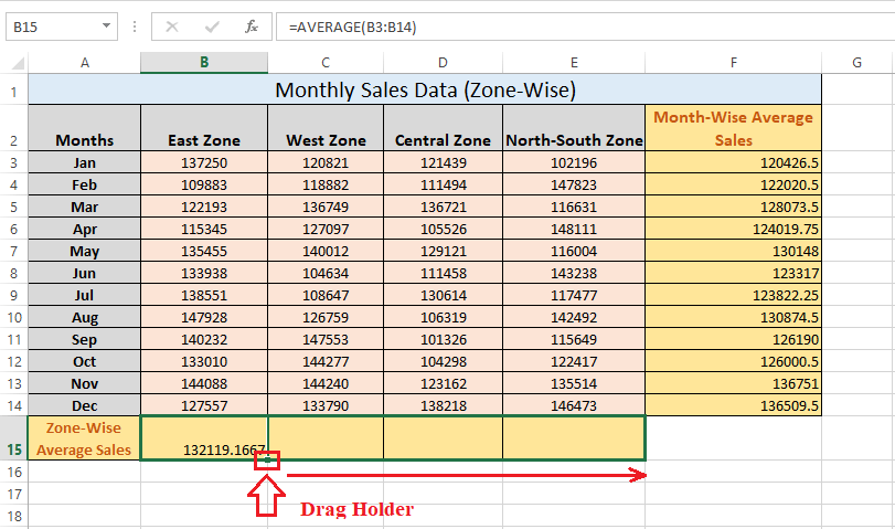
This immediately provides the average sales for the rest of the zones by applying the appropriate AVERAGE function in corresponding cells.
Example 3: Calculating the Average for Initial (top) n Values
We can use the AVERAGE function to calculate the average value for top n numerical values. It can be performed by combining the AVERAGE function with the LARGE function.
For instance, let us consider the following Excel sheet with some marks given to employees in an interview. We want to calculate the average marks achieved by each employee only in the top three rounds without including the practical marks.
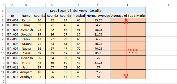
In the above example, we can usually find out the average marks for each student in all rounds and a practical by using the process discussed in example 1. However, to calculate the average marks only for the top three rounds, we need to use the AVERAGE function with the LARGE function like this:
=AVERAGE (LARGE(C3:F3, {1, 2, 3} ) )
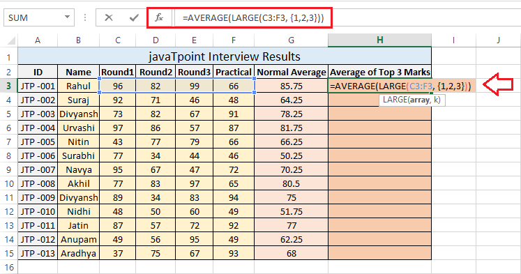
Upon pressing the Enter key, the function returns the average value of the top three marks scored by an employee out of all four marks, which is shown below:
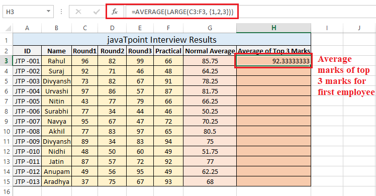
Now, we have obtained the average marks of the top three rounds for the first employee. Next, we need to drag a result cell to the rest of the result cells.

This will provide the average result of the top three marks for all the other employees.

That is how we can use the AVERAGE function in Excel.
Some Important Points to Remember
To successfully apply the AVERAGE function in Excel, we must remember the following facts:
- By the definition of average, the supplied values (or numbers) are first added together, and then its sum is divided by the total numbers of supplied values.
- A total number of 255 individual arguments can be supplied to the AVERAGE function.
- Inputs or arguments can be supplied directly into the AVERAGE function, cell references, or named ranges.
- The Excel AVERAGE function ignores all such arguments supplied as text, text values, empty cells, and logical values like TRUE/ FALSE.
- The AVERAGE function only understands numeric values or their references; thus, it returns # VALUE! Error if the supplied values cannot be interpreted as numeric values.
- If all the supplied arguments in the AVERAGE function are non-numeric, the function returns the #DIV/0! Error.
- The zero values or cell references with zero values are counted in the AVERAGE function.


