Excel array formula
Array formula is an extremely powerful but difficult one formula in Excel. A single array formula can perform multiple calculations at once. Basically, it is a type of formula that allows the users to perform any operation of multiple values rather than a single value. The returned value from the array formula can be an array item or an array of items.
Usually, we perform operations on a single value or range of values. An array formula should be surrounded between curly braces ({}). In this chapter, you will learn the array formula in Excel and how you can perform it on Excel data.
What is an array?
An array is a collection of multiple values or you can say that an array contains more than one value. The array values reside inside the curly braces ({}) in Excel. Whenever you want to perform any operation on an array, put it inside the curly braces. Even for array formula, you need to put the formula inside curly braces.
An array formula is not an easy task to perform on Excel data. You have to learn the way to perform this.
How to enter an array formula?
Enter a simple formula and use the Ctrl+Shift+Enter key rather than Enter key to get the result. The Ctrl+Shift+Enter key converts the simple formula to an array formula at the resultant time.
Basically, it evaluates the simple formula as an array formula and returns the result accordingly. Entering an array formula manually to a cell does not work. Manually entering an array formula does not return any result.
Representation of array
An array looks like {10; 20; 30} or {“UP”, “MP”, “UK”}. Here, you will notice that – we have used semicolon (;) and comma (,) to separate the values inside an array. Both have different meanings in their usage.
The array values that are separated by the semicolon, represent the vertical range of data in an Excel sheet. While for horizontal range, a comma is used to separate the values inside the array. Both the examples for the one-dimensional arrays. A two-dimensional array uses both semicolons and commas for horizontal and vertical ranges in an Excel sheet.
Vertical range ({10; 20; 30})
A vertical range represents the values of a column. Basically, if you want to represent the value of a column as array, use the vertical range for it in an Excel sheet.
For example, you can understand the following array values {10; 20; 30} in column A that might be placed in A1, A2, and A3.
Horizontal range ({“UP”, “MP”, “UK”})
A horizontal range represents row data. A horizontal range refers to the values that appeared inside a row in an Excel sheet. For example, you can understand the following array values {“UP”, “MP”, “UK”} in row1, i.e., A1, B1, and C1.
Example 1: Array formula implementation
Without an array formula
Without an array formula, multiple values like this (A2:A9) is just a range of cells containing values in cells selected from A2 to A9.
See a simple scenario for a simple dataset in which we will show you a difference of simple formula and array formula. We have taken some products with their price and quantity to order.
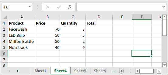
Step 1: We have the total price of each product. We will now find the total price of all products.

Step 2: We can minimize this lengthy process into one by using the array formula. Write the following formula to find the total of all processes and hit the Ctrl+Shift+Enter key.
=SUM(B2:B5*C2:C5)
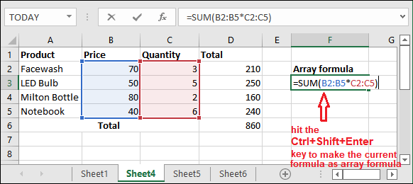
Currently, this formula is like the simple formula, but when you press the Ctrl+Shift+Enter key, this written formula will become an array formula {=SUM(B2:B5*C2:C5) automatically.
“Remember – do not press the Enter key after entering the formula in cell.“
Step 3: See in the below screenshot where you see that we have got the same result, as we found by following a large process.
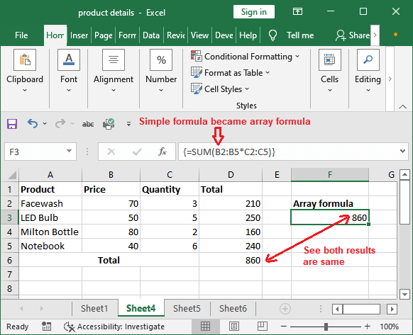
Step 4: In case you press the Enter key instead of Ctrl+Shift+Enter, you may either get #VALUE! Error or an incorrect value.
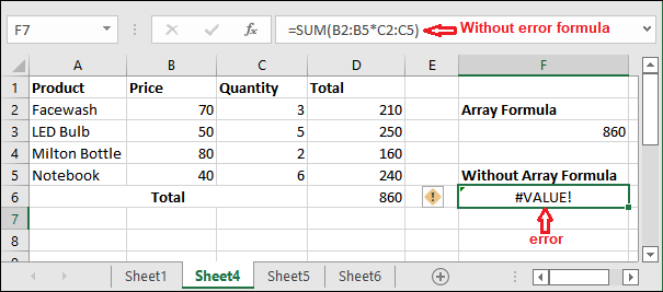
We have not got the correct resultant value (error) because the formula has not changed to an array formula.
Example 1
We have taken an example below in which you can see that the data in (B2:B13) is the sale of one year for each month. The data in (C2:C13) is for the expense of one year from month January to December. Column D contains the profit/loss of each month whose total is placed in the end (in cell D14).
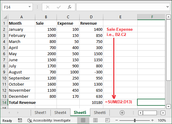
For calculating the yearly profit/loss, we have to first find the per month revenue and then the total sum of the calculated revenue. It can be a lengthy process for a large set of data. We can minimize this process and make it easy by using an array formula. The array formula makes this process short.
Multi-cell array formula
The multi-cell array formula reduces the lengthy calculation. By using the array formula, you can get the final result (yearly revenue) at once. You need only one array formula instead of this long calculation.
If you try this formula without an array formula, you have to use the formula to calculate the yearly revenue as given below and press the Enter key.
=SUM(B2:B13*C2:C13)
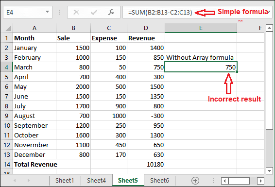
But this will either return you an incorrect value or #VALUE! Error. So, do not use formula like this. If you want to perform an operation like this formula, then press the Ctrl+Shift+Enter key to make the normal formula an array formula.
Array formula
The array formula will be as follows for the above formula.
{=SUM(B2:B13*C2:C13)}
An array formula is surrounded between the {} (curly braces). You do not write an array formula directly in a cell to get the result. It will return nothing, neither error nor incorrect result. So, you need to follow the steps as given below:
Step 1: Write the simple formula and hit the Ctrl+Shift+Enter key to get the result as an array formula.

The Ctrl+Shift+Enter key converts a simple formula to an array formula.
Step 2: See the result for an array formula this time, which is same as we achieved by a lengthy calculation.

“You can also press Ctrl+Shift+Enter key instead of Enter key with normal formula to get the result for array formula.”
Why use array formulas in Excel?
With the help of Excel formula, the users can perform calculations on Excel data to do complex tasks. It reduces the efforts of users to perform lengthy calculations to get the final result by using the array formula. A single array formula replaces the various unusual formulas.
You can use the array formula for tasks for this it is good for:
- For example, sum the N largest or smallest values in a range that meets with certain conditions.
- Calculate the revenue for entire years from the data of each month sales and expenses. In such a situation, an array formula ignores calculation profit and lost then sum of total and provide result with a single formula.
Excel array constant
An array constant is a set of static values. As array constants have static values, they never change when you copy a formula to other cells. In MS Excel, there are three types of an array constant.
- Horizontal array constant
- Vertical array constant
- 2D array constant
Horizontal array constant
A horizontal array constant refers to the values in a row. To create a horizontal array constant, type the value separated by a comma enclosed between curly braces ({}).
For example, {1, 2, 3, 4}
To create a horizontal array constant, select the corresponding number of cells in a row and enter the following array in the formula bar.
={1,2,3,4}

Now, hit the Ctrl+Shift+Enter key and see how the horizontal array constant looks.

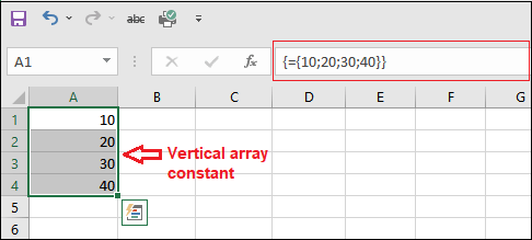
Vertical array constant
A vertical array constant resides in an Excel column. It means the values of vertical array constant refers to the values in a column. To create a vertical array constant, type the value separated by semicolon enclosed between curly braces ({}).
For example, {11; 22; 33; 44}
To create a horizontal array constant, select the corresponding number of cells in a row and enter the following array in the formula bar.
={10; 20; 30; 40}

Now, hit the Ctrl+Shift+Enter key and see how the horizontal array constant looks.
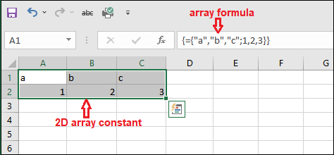
2D array constant
2D array constant is a combination of vertical and horizontal array constant. As it is a combination of horizontal and vertical constants, it uses both semicolon and comma to represent the row and column values.
For example, 2D array constant uses semicolon to separate each row value and comma to separate each column value, i.e., {“a”, “b”, “c”; 1, 2, 3}.
To create a 2D array constant, select the corresponding number of cells in both row and column. Then, enter the following array in the formula bar.
={“a”, “b”, “c”; 1, 2, 3}

Now, hit the Ctrl+Shift+Enter key and see how the horizontal array constant looks.