
Excel Absolute Referencing
Microsoft Excel, also known as Excel, is an extremely powerful spreadsheet program developed by the Microsoft Company. Using Excel, users access multiple worksheets to record large amounts of data within one or more cells. Additionally, Excel has a different range of built-in functions to help us apply various operations or calculations on recorded data to achieve financial analysis or desired output.
Although most formulas can work with numerical values directly assigned to them, we often use cell references to access desired values that we want to supply in specific formulas. Using cell references is useful because the formula automatically updates the corresponding output in the resulting cells accordingly if we change the values recorded. There are mainly three types of cell references, namely relative, absolute and mixed.

In this tutorial, we discuss a brief introduction to Excel Absolute Referencing. We also discuss the step-by-step procedures to create or use an absolute reference in our Excel worksheet with the help of relevant examples. Before we look at Absolute Reference in Excel, let us first introduce Excel Cell Reference.
What is a Cell Reference?
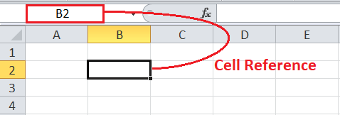
An Excel cell reference refers to the address or name of the corresponding cell or a range of multiple cells. It usually consists of the corresponding column name followed by the specific row number. A cell reference tells Excel formulas where to look for the data/value used in the formulas. In Excel, we can refer to cells in the same sheet, another sheet, another workbook, and other supported programs.
What is an Absolute Reference in Excel?
By default, Excel uses relative references, which means that the cell reference changes based on the relative position of the row and column when it is copied to another cell or range. However, there may be cases when we may need to fix the addresses of some cells to get specific outputs. After fixing the cell references, we can ensure that they do not change even after copying them to another location. This is where Excel Absolute Referencing comes into play.
By definition, “Excel Absolute Reference refers to a’ locked’ reference so that the address of its corresponding row and column does not change when copied“.
An absolute reference in Excel represents an actual fixed location or address on the worksheet. So, when we want to fix the position of the desired cell in an Excel formula so that its position remains constant while copying it to another location, we make the corresponding cell in the formula absolute.
When do we need to use Absolute Cell References in Excel?
When working in Excel, we come across a wide range of use-cases where we have to use absolute references to get the desired results, regardless of the field or industry we are working on. Some of the common cases when we commonly use absolute references for efficient calculation and reporting are as follows:
- When calculating the sales taxes based on the certain fixed rate for invoices of different items
- When using a fixed price per unit
- When implementing a single percentage for individual years to calculate annual profit targets in projects
- When changing prices or units for multiple cells values at certain fixed measurements
- When referring to fixed-availability rates for each resource while managing projects
- When using the relative references for a column and absolute reference for a row to match the column calculation in our referenced cells to use its value in other desired data tables or a range
How to create or make an Absolute Cell Reference?
We should include the dollar sign ($) before the column name and row number for desired cell reference to make it absolute. Depending upon the use-cases, we may need either to fix an individual cell or an entire range. Let us discuss both the cases:
Creating/ Making a cell Absolute
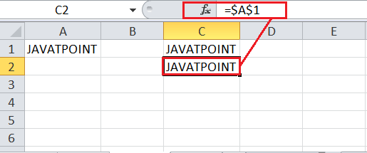
When we need to make a single cell an absolute cell, we must insert a dollar sign before the column name and row number. This will change the relative reference into an absolute reference.
For example, an absolute reference to cell A1 will be as below:
=$A$1

If we copy the cell to the other cell below, the absolute reference remains the same and gives the same output.
Creating/ Making a range Absolute
When we need to make an entire range absolute, we must add a dollar sign to each cell reference in the range. For example, if we have a range A1:B7 to be used in the form of an absolute reference. We need to include the dollar sign in the following way:
=$A$1:$B$7
That way, we fix the column letters and row numbers for the entire range.
Note: Instead of manually adding the dollar sign ($), we can also press the F4 function key once after placing the cursor in the specific cell reference in the formula bar. This will immediately add a dollar sign to a particular cell reference, making it absolute. Pressing the F4 function key multiple times will toggle between other types of cell references.
How to use Absolute Referencing in Excel?
We need to perform the below steps to use the absolute referencing in Excel properly:
- First, we must select a resultant cell to insert a formula and type the equal sign (=) to start the formula.
- Next, we need to start typing the function name and select it from the list by pressing the TAB key on the keyboard. After that, we must supply the respective arguments as per syntax.
- In the next step, we need to click between the cell in the formula bar that we want to make an absolute. Also, we must press the F4 function key once that converts the relative cell reference into an absolute reference. We can do this for all the desired cells or a range in the formula bar.
- After making the desired cells/ range absolute, we must press the Enter key on the keyboard. Now, we can copy the formula to any other location on the sheet without automatically converting it by Excel.
Let us now understand the concept of absolute reference better with the help of the following examples:
Absolute Referencing in Excel: Example 1
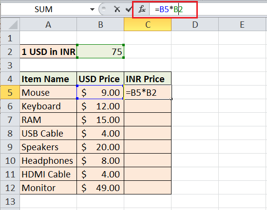
Consider the following sheet as an example data set where we have prices of different items in USD ($).
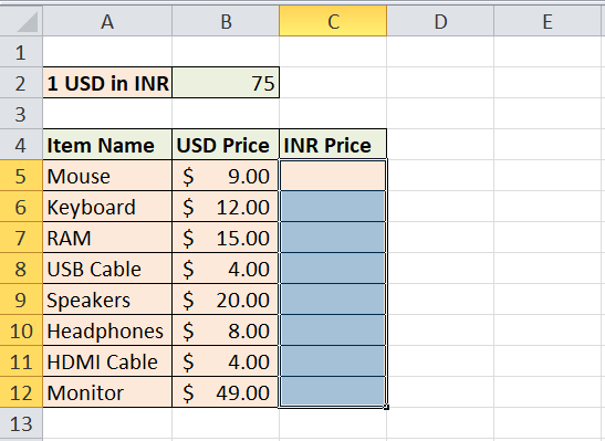
We need to convert these prices from USD to INR in a column (C) next to it. Suppose 1 USD equals approximately 75 INR, recorded in cell B2 in the sheet. In that case, we need to multiply the recorded prices of different items with cell B2. So, we need to fix cell B2 in the multiplication formula while keeping all other cells relative or default.
The steps to convert or change the recorded prices from USD to INR by using the multiplication formula are listed below:
- We first need to select cell C5 and type an equal sign (=) to start the formula. Next, we select the respective cell B5, type the multiplication operator (*), and select cell B2. After that, we press the Enter key to get the corresponding result for the first item.

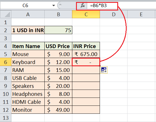
In the above image, we can see the price of the first item in INR. The result is correct for the first item. However, if we copy the formula into other cells below cell C5 to get the INR prices for the other items, we get the incorrect prices. When we copy the formula from C5 to C6, the cell references automatically change for given cells B5 and B2 (as shown in the following image). But, we have to fix cell B2 to get the appropriate results, so we make it absolute first.
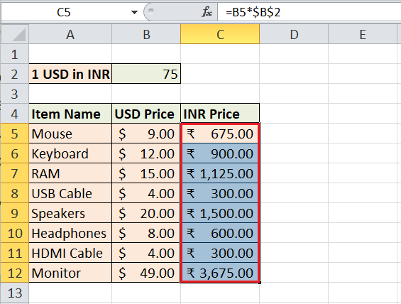
- Before copying the formula into other cells, we again select the cell where we have initially inserted the formula, i.e., cell C5. Then, we go to the formula bar and click or place the cursor in between cell B2.
- In the next step, we press the F4 function key once. This immediately changes the reference from B2 to $B$2 in the cell C5, and the entire formula changes from (=B5*B2) to (=B5*$B$2), as shown below:

- Once the cell reference has been converted into the absolute reference, we must press the Enter key. Lastly, we can drag or copy-paste the formula into other cells below C5, and the prices will be converted from USD to INR correctly.
Absolute Referencing in Excel: Example 2
Consider the following sheet as an example data set where we list some grocery items with their prices and purchased quantities.

Our example sheet shows that we have the fixed GST (Goods and Service Tax Rate) rate of 5% for each item. For calculating the Net Prices (Total Price including the GST), we first need to calculate the GST price for each item and then include this in the respective total prices.
The steps to calculate the total prices, including the GST for each item, are listed below:
- First, we need to calculate the total price for each item without the GST in column E. So, we select cell E4 to record the total for the first item, excluding the GST. We do this by multiplying the number of quantities purchased with the respective price, as shown below:

After applying the multiplication formula, we press the Enter key and drag the formula to other column cells to get the respective total prices for each item.

Since there is no fixed value in the multiplication formula, we don’t need to use the absolute reference. - In the next step, we need to calculate the GST price for each value. Since the GST rate is fixed (cell G1), we must use the absolute reference here. So, we calculate the GST for the first item by multiplying the total price with the GST rate. Also, we make the cell with GST rate an absolute reference in the following way:

After pressing the Enter key on the keyboard, we get the GST price for the first item. Since we have the absolute reference for the desired fixed cell ($G$1), we can copy or drag the formula to other cells below in column F to get the GST prices for all items. Thus, we keep the fixed GST rate constant in cell G1, while the relative reference for column E changes accordingly.

- After calculating the GST prices for items, we can calculate their respective total price, including the GST. For this, we must add the total price with the GST price in the following way:
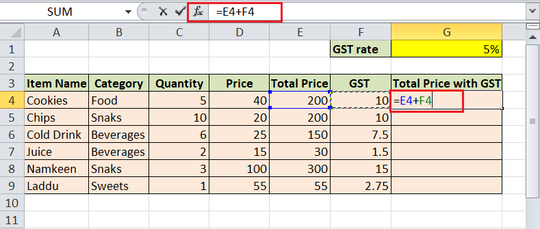
Since both the cells in the formula are relative (changing values cells), we can drag or copy-paste the formula into other cells to get the total prices for the other items, including the GST.

An alternate to Excel Absolute Referencing: Named Range
In Excel, a named range is an alternative to an absolute reference. We can name any desired cell or a range accordingly and use it in our formulas. This way, we can make our formulas easier to understand. Depending on our requirements, we can create multiple named ranges in a single sheet. For this, we can use the Name Manager and create, edit or delete the desired named range accordingly.
For example, suppose we have salary data of some employees, and we want to include the additional bonus of 1500 INR with each respective salary. The data is structured in an Excel sheet in the following way:

We need to fix cell C1 in the formulas in the above sheet. So, we name this cell as a BONUS using the Name Manager (Formulas > Name Manager).

After that, we select the resultant cell C4 and insert the formula (Salary + Bonus) to calculate the total salary for the first employee.
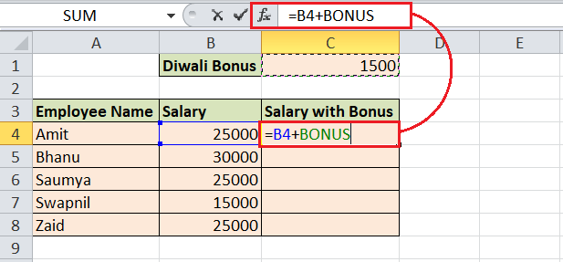
After pressing the Enter key, we get the first employee’s desired result (total salary).

Now, we can drag or copy-paste the formula in other cells below C4 to get the total salary of other employees. Since we have named the cell C1 as BONUS, it does not change automatically in other resultant cells (C5, C6, C7, and C8).

Similarly, we can also assign a name for the desired range and use it in the corresponding formulas. This concept works similarly to the Excel Absolute Referencing.
Important Points to Remember
- We fix both the respective column and the row when using the absolute reference. If only a row or column is fixed by placing a dollar sign before it, the respective cell reference will be called the ‘mixed reference’.
- Excel absolute reference does not automatically change irrespective of the movement of the respective formula in upward, downward, leftward or rightward direction.
- When pressing the ‘F4’ shortcut key to change the cell reference, we may first need to activate the function keys by pressing the ‘Fn’ function key for specific keyboards.


