Convert rows to columns

An Excel worksheet contains the data in rows and columns. Excel lets users to transpose the data if they want to re-arrange the data by rotating it from row to column. It allows to convert the data stored in Excel rows to columns, and rows become columns. Use the Transpose feature of Excel for it.

This chapter will describe to use the Excel Transpose feature to re-arrange the rows data to columns. Using this, you can quickly switch the data from rows to columns.

Why convert from rows to columns

Sometimes, you store data in Excel cells correctly, but it does not look good to your eyes to analyze it due to the wrong cell placement of data. You find difficulty in reading and analyzing the data. You realize it when you set up the data in Excel and created a worksheet with large data. For example,

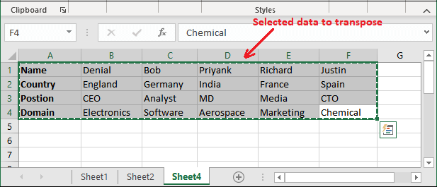
Name	Denial	Bob	Priyank	Richard	Justin
Country	England	Germany	India	France	Spain
Position	CEO	Analyst	MD	Media	CTO
Domain	Electronics	Software	Aerospace	Marketing	Chemical

How to resolve it?

There is no need to re-enter the whole data and put effort once again. Excel offers a Transpose feature for it.

If you find this data difficult to read, Excel allows converting the rows data to columns and vice versa. By transforming the Excel data, you can get the data a new look and the way of seeing the data is changed.

See if you transform the Excel data, it will look like this –

Name	Country	Position	Domain
Denial	England	CEO	Electronics
Bob	Germany	Analyst	Software
Priyank	India	MD	Aerospace
Richard	France	Media	Marketing
Justin	Spain	CTO	Chemical

You can store the data in Excel cells however you want, and even change it later using Excel’s transpose feature.

Tips for transposing data in Excel

Following are some helpful tips for readers that they should know –

1. Your data can include formulas. Excel does not lose the formulas and their resultant values when transposing the data.
2. Excel automatically update the formulas by updating the references of cells inside the formula and keeps the values same.
3. If you just want to see the data from different angles, we will suggest you create a pivot table. It allows to drag the fields from rows to columns.
4. If the Transpose feature is not available, you can convert the Excel table data using the Convert to Range button available inside the Table tab.
5. Besides this, Excel users can also use the transpose() function to rotate the rows data to column data.

Note: You can find the transpose feature inside Excel Paste Special panel.

Methods to convert rows to columns

We are having two different ways to convert the data from rows to columns. You can choose any one method. These are –

1. Transpose the Excel data using Paste Special
2. Transpose the rows to columns using TRANSPOSE formula

Both methods are completely different from each other.

Transpose the Excel data using Paste Special

We are using the transpose feature available inside the Paste Special panel to convert the rows to columns. It is a static method to transpose data. If you change anything in the original data or delete it, it will not reflect in transposed data.

Look at the steps for how to use this method to transpose data –

Step 1: Select the range of cells data you want to transpose and click Ctrl+C to copy.

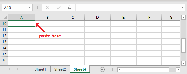
Step 2: Go to the new location in the sheet where to paste the transposed data.

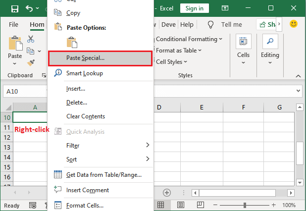
Step 3: Now, right-click and select Paste Special from the list.

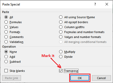
Step 4: Mark the transpose checkbox inside this Paste Special panel, as shown in the below image, and click OK.

Step 5: You can now see that the rows data is successfully transposed to columns.

Step 6: See both data together before and after transpose and see how they look different.

This method is not limited. You can transpose any number of rows to columns. For example, one or more. Now, let’s check out the next method (TRANSPOSE formula).

If original data value is changed

This method is a static method to transpose the data. If you change in original data, it will not reflect on transposed data. Look at an example for it too:

For example, you change the value of C2 cell (from Germany to USA), it will not change inside the transposed data (C10 cell).

If original data has deleted

As we told you that it is static, not a dynamic method. Thus, even if you delete the original data, the transposed data will be the same and nothing will happen.

Look at an example for it in which we have deleted entire original data but its corresponding transposed data has not been deleted:

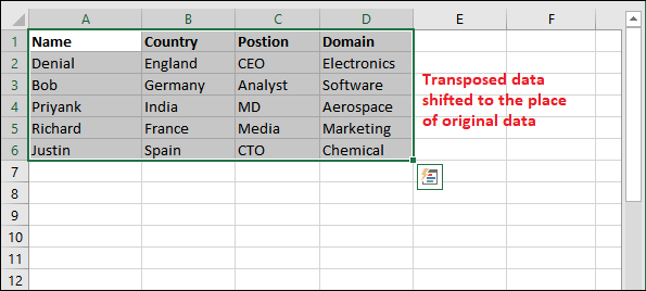
Step 7: After transposing the data successfully from rows to columns, you can delete the previous data and even shift the transposed data to there.

Transpose the rows to columns using TRANSPOSE formula

This time we are using the inbuilt Excel TRANSPOSE formula to convert the rows to columns. To use this function, you should know the syntax of it and how to use it. It is a dynamic solution to change the rows to columns. So, when

TRANSPOSE function

The TRANSPOSE function is an Excel function that helps to change the row orientation to row. The data rows become columns and data columns become rows. It is a very simple and easy to use function to transform the large range of data in Excel.

This array parameter contains the range of cells to be transposed.

Steps to transpose data using TRANSPOSE() function

Look at the steps for it with an example –

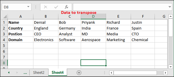
Step 1: Here, we have initial data whose formation we want to change.

Step 2: Count the number of rows and columns that will replace to each other after transforming. Currently, here are four rows and six columns that will become six rows and four columns.

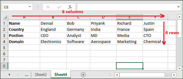
Step 3: Select six blank rows and four blank columns. It is must to select the same number of rows and columns for conversion.

E.g., 4 rows 6 columns = 6 rows 4 columns

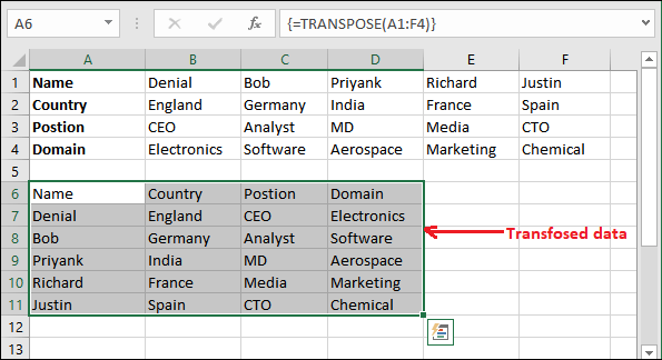
Step 4: Now, type the following formula in the first selected cell without cancelling section. Here we have put the formula inside the A6 cell.

=transpose(A1:F4)

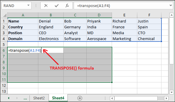
A1:F4 is the data selected to transpose (from row to column).

Step 5: Press the Ctrl+Shift+Enter key if you are not using Office 365 and get the transposed data. See the data converted from rows to columns.

Tip: Press the Enter key if you are using Office 365 online to get the correct transposed result on it.

If original data value is changed

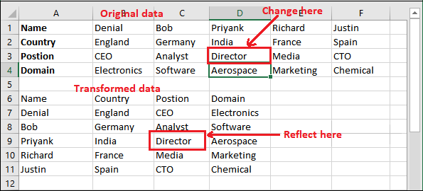
TRANSPOSE(() is a dynamic formula. If you change in original data, it will reflect on transposed data. Look at an example for it too:

For example, you change the value from MD to Director in D4 cell, it will automatically change in its corresponding transformed cell (C9 cell).

If original data has deleted

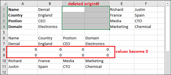
As we told you that TRANSPOSE(() is a dynamic formula. Thus, if you delete the original data, the transposed data will also be changed and the values become 0.

Look at an example for it in which we have deleted column C and column D from original data and their corresponding values become 0 in transposed data:

Use Transpose feature of Paste Special

You can make the process faster by directly using the Transpose method of Paste Special feature. Paste Special has a Transpose option inside it. You can directly access it from Paste Special and improve the process. To learn this process to transpose data, follow the below steps –

Step 1: We have this initial data. Here, select the range of cells data you want to transpose and click Ctrl+C to copy.

Step 2: Go to the new location in the sheet where to paste the transposed data.

Step 3: Now, right-click on this cell and select Paste Special from the list and click the Transpose feature button of Paste Special.

Step 4: It will convert the rows data to columns data. See the screenshot for transposed data below:

Difference between Paste Special and TRANSPOSE() function

Both methods are used for transposing the Excel data ad they produce the same results. There is a big difference between them.

The first method: Paste Special is a static method to transpose (convert rows to columns) the data. Nothing will happen in transpose data if you change something in original data.

Another method: TRANSPOSE() function is a dynamic method to transpose the data from rows to columns. If you make changes in original data, its related transposed data will reflect. Also, if you delete the original data, its transposed data will also be deleted automatically.

When use Paste Special

1. If you want to continue the original formatting (like bold text, text formatting, and all), transpose Paste Special method is good for you.
2. Paste Special transpose the Excel data from row to column along with original formatting.
3. The transpose Paste Special method does not link the transposed data with original data. So, if you make changes in original data, it does not reflect on transposed data.
4. You can easily edit or delete the transposed data converted using transpose Paste Special method without any interruption.

When use TRANSPOSE() function

1. The TRANSPOSE() function links the transposed data with original data. So, if you make changes in the original data, it automatically reflects on transposed data.
2. TRANSPOSE() function removes the formatting after converting rows to columns.
3. Do not use this method if you want to keep formatting as in original data after transposing.
4. You cannot edit or delete the transposed data converted using the TRANSPOSE() function. If you try to edit/delete it, it will show an error like – You cannot change a part of an array.

---