Chart with Arrows in Excel
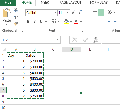
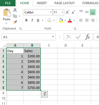
Now we will create a simple bar chart from the Excel file as shown below. Select the entire data:
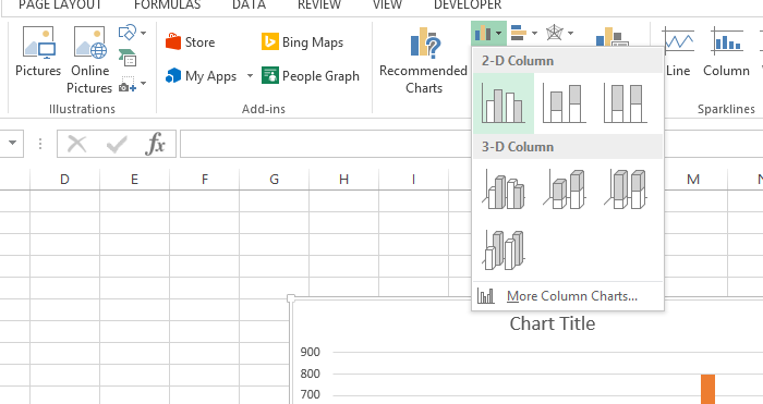
From the Insert tab from Excel, select insert column chart:

Select 2d column:
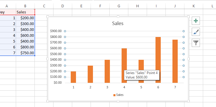
Unselect Day from select data:

Chart will look like this now:
Now we will have to convert these columns to arrows. Insert > shapes > arrow:

Drag the space on Excel to draw arrow:

After selecting the arrow press ctrl + c to copy the arrow. Then select all the bars in the chart:
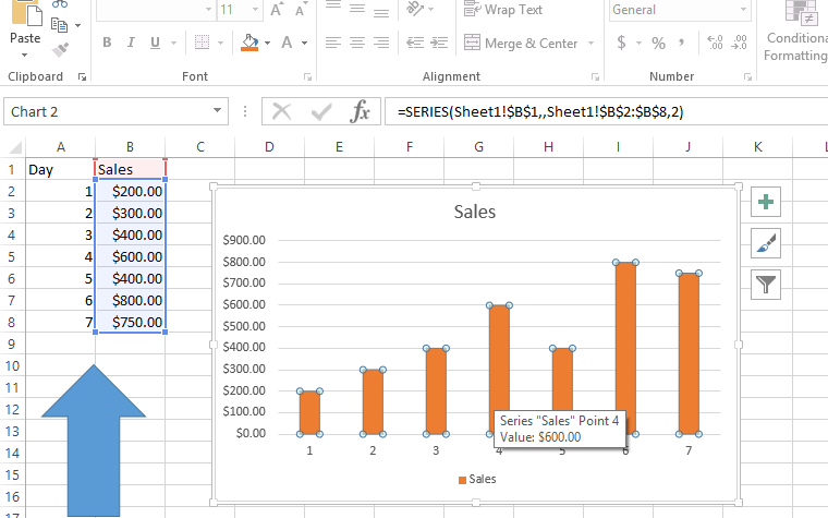
After selection just type ctrl + v to paste all the shapes to the bars of the chart and then it will just look like the below arrow chart.
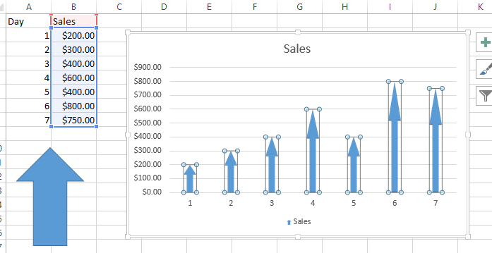
Then we can remove the extra arrow.
Template
You can download the Template here – Download
Further reading:
Basic concepts
Getting started with Excel
Cell References


