ISERROR function
This example illustrates the ISERROR function in Excel.
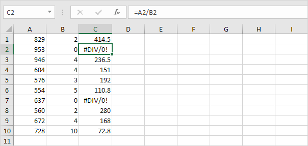
1. For example, Excel displays the #DIV/0! error when a formula tries to divide a number by 0.

2. The ISERROR function in Excel checks whether a value is an error and returns TRUE or FALSE.

3. Add the IF function. If a cell contains an error, the value 5 is returned. If not, the value 100 is returned.

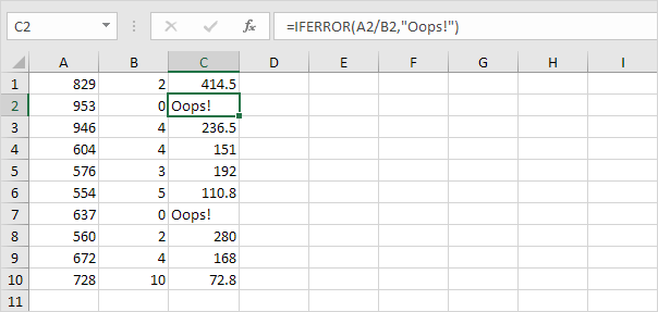
4. Use the IFERROR function to return the result of a formula (if there’s no error) or an alternative result, such as text (if there’s an error).

5. Use COUNT, IF and ISERROR to count the total number of errors in a range of cells.

Note: this is an array formula. You can finish an array formula by pressing CTRL + SHIFT + ENTER. Excel adds the curly braces {}. Visit our page about Counting Errors for detailed instructions on how to create this array formula.
Next Chapter: Array Formulas


